Automatically plot an epi_df or epi_archive
Usage
# S3 method for class 'epi_df'
autoplot(
  object,
  ...,
  .color_by = c("all_keys", "geo_value", "other_keys", ".response", "all", "none"),
  .facet_by = c(".response", "other_keys", "all_keys", "geo_value", "all", "none"),
  .base_color = "#3A448F",
  .facet_filter = NULL,
  .max_facets = deprecated(),
  .max_keys = 10,
  .interactive = FALSE,
  .facet_to_dropdown = FALSE
)

# S3 method for class 'epi_archive'
autoplot(
  object,
  ...,
  .base_color = "black",
  .versions = NULL,
  .mark_versions = FALSE,
  .facet_filter = NULL,
  .max_keys = 6,
  .interactive = FALSE,
  .facet_to_dropdown = FALSE
)

# S3 method for class 'epi_df'
plot(x, ...)

# S3 method for class 'epi_archive'
plot(x, ...)
Arguments
- object, x
An
epi_dforepi_archive- ...
<
tidy-select> One or more unquoted expressions separated by commas. Variable names can be used as if they were positions in the data frame, so expressions likex:ycan be used to select a range of variables.- .color_by
Which variables should determine the color(s) used to plot lines. Options include:
all_keys- the default uses the interaction of any key variables including thegeo_valuegeo_value-geo_valueonlyother_keys- any available keys that are notgeo_value.response- the numeric variables (same as the y-axis)all- uses the interaction of all keys and numeric variablesnone- no coloring aesthetic is applied
- .facet_by
Similar to
.color_byexcept that the default is to display each numeric variable on a separate facet- .base_color
Lines will be shown with this color if
.color_by == "none". For example, with a single numeric variable and faceting bygeo_value, all locations would share the same color line.- .facet_filter
Select which facets will be displayed. Especially useful for when there are many
geo_value's or keys. This is a <rlang> expression along the lines ofdplyr::filter(). However, it must be a single expression combined with the&operator. This contrasts to the typical use case which allows multiple comma-separated expressions which are implicitly combined with&. When multiple variables are selected with..., their names can be filtered in combination with other factors by using.response_name. See the examples below.- .max_facets
![[Deprecated]](figures/lifecycle-deprecated.svg)
- .max_keys
Maximum number of key combinations to display. If the data contains more key combinations than this limit, a random sample of size
.max_keysis displayed, and a warning is issued. Set toInfto display all keys. Subsampling is not performed if.interactive = TRUE(though a similar limit may be applied to initial legend visibility) when.facet_to_dropdown = FALSE.- .interactive
Logical. If
TRUE, returns an interactiveplotly::ggplotly()widget instead of a staticggplot2::ggplot()object. This is especially useful for exploring datasets with many keys. Default isFALSE.- .facet_to_dropdown
Logical. If
TRUE, and.interactive = TRUE, any facets will be converted into a dropdown menu. This is useful for maximizing screen real estate when there are many facets. Default isFALSE.- .versions
Select which versions will be displayed. By default, a separate line will be shown with the data as it would have appeared on every day in the archive. This can sometimes become overwhelming. For example, daily data would display a line for what the data would have looked like on every single day. To override this, you can select specific dates, by passing a vector of values here. Alternatively, a sequence can be automatically created by passing a string like
"2 weeks"or"month". For time types where thetime_valueis a date object, any string that is interpretable bybase::seq.Date()is allowed.For
time_type = "integer", an integer larger than 1 will give a subset of versions.- .mark_versions
Logical. Indicate whether to mark each version with a vertical line. Note that displaying many versions can become busy.
Value
A ggplot2::ggplot object, OR plotly::plotly object if .interactive = TRUE
Examples
# -- Use it on an `epi_df`
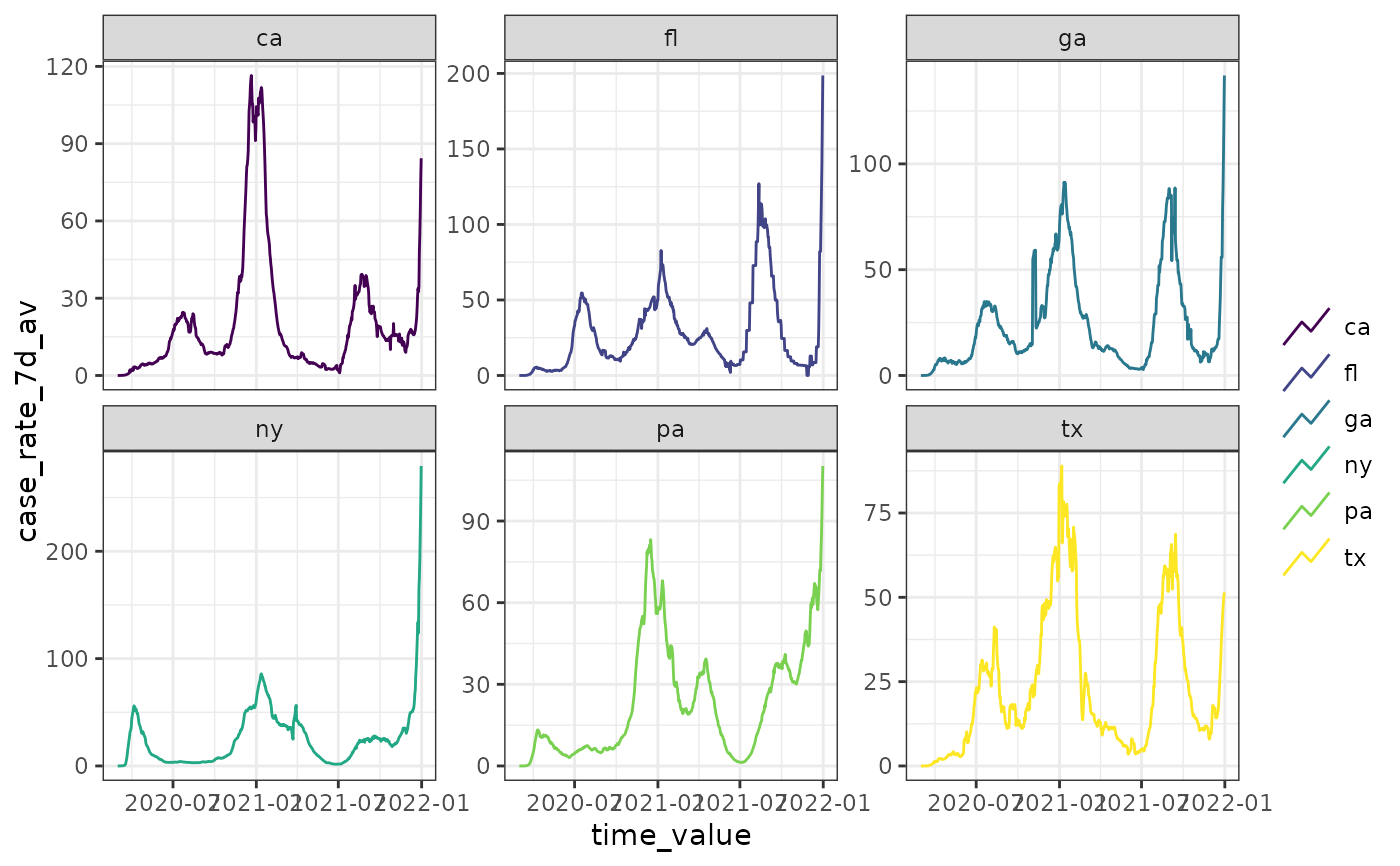
autoplot(cases_deaths_subset, case_rate_7d_av, death_rate_7d_av)
#> Warning: Too many key combinations to display clearly. Showing 10 of 12.
#> → To plot all keys, use `autoplot(..., .max_keys = Inf)`.
#> → To explore all keys interactively, use `autoplot(..., .interactive = TRUE)`.
#> → To plot specific keys, use `autoplot(..., .facet_filter = ...)`.
 # Launch interactive version in web browser:
autoplot(cases_deaths_subset, case_rate_7d_av, death_rate_7d_av,
.interactive = TRUE
)
# Use dropdowns instead of facets for interactive plots
autoplot(cases_deaths_subset, case_rate_7d_av, death_rate_7d_av,
.interactive = TRUE, .facet_to_dropdown = TRUE
)
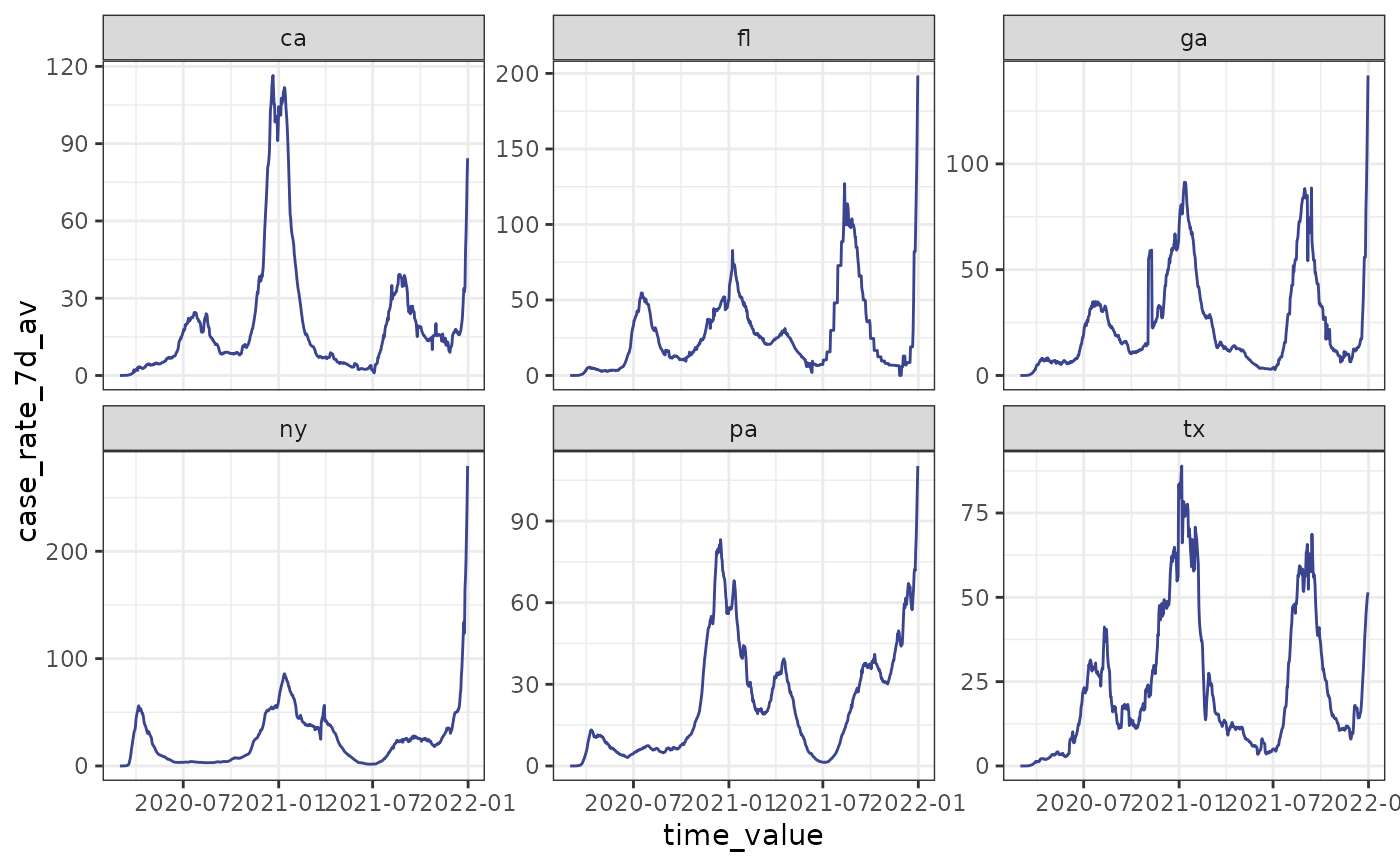
autoplot(cases_deaths_subset, case_rate_7d_av,
.color_by = "none",
.facet_by = "geo_value"
)
# Launch interactive version in web browser:
autoplot(cases_deaths_subset, case_rate_7d_av, death_rate_7d_av,
.interactive = TRUE
)
# Use dropdowns instead of facets for interactive plots
autoplot(cases_deaths_subset, case_rate_7d_av, death_rate_7d_av,
.interactive = TRUE, .facet_to_dropdown = TRUE
)
autoplot(cases_deaths_subset, case_rate_7d_av,
.color_by = "none",
.facet_by = "geo_value"
)
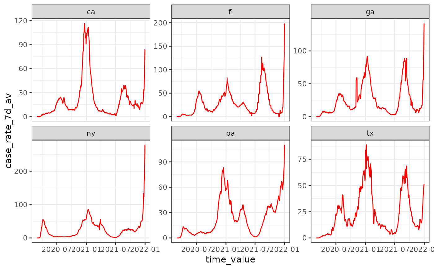
 autoplot(cases_deaths_subset, case_rate_7d_av,
.color_by = "none",
.base_color = "red", .facet_by = "geo_value"
)
autoplot(cases_deaths_subset, case_rate_7d_av,
.color_by = "none",
.base_color = "red", .facet_by = "geo_value"
)
 # .base_color specification won't have any effect due .color_by default
autoplot(cases_deaths_subset, case_rate_7d_av,
.base_color = "red", .facet_by = "geo_value"
)
# .base_color specification won't have any effect due .color_by default
autoplot(cases_deaths_subset, case_rate_7d_av,
.base_color = "red", .facet_by = "geo_value"
)
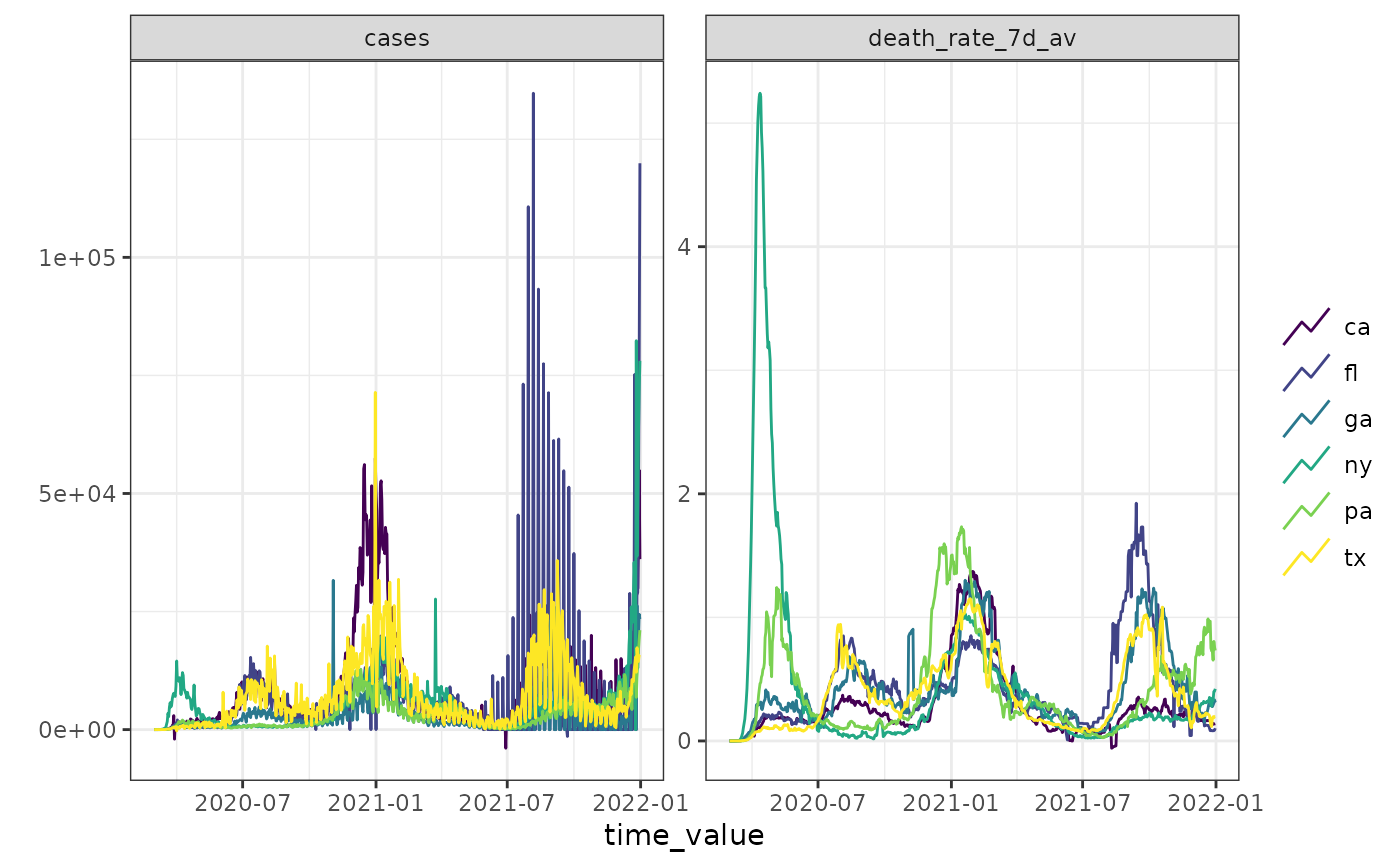
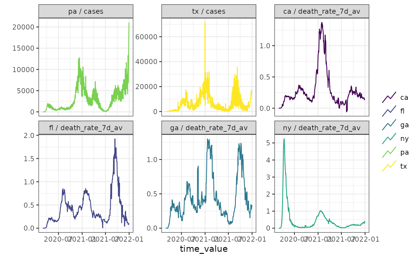
 # filter to only some facets, must be explicitly combined
autoplot(cases_deaths_subset, cases, death_rate_7d_av,
.facet_by = "all",
.facet_filter = (.response_name == "cases" & geo_value %in% c("tx", "pa")) |
(.response_name == "death_rate_7d_av" &
geo_value %in% c("ca", "fl", "ga", "ny"))
)
# filter to only some facets, must be explicitly combined
autoplot(cases_deaths_subset, cases, death_rate_7d_av,
.facet_by = "all",
.facet_filter = (.response_name == "cases" & geo_value %in% c("tx", "pa")) |
(.response_name == "death_rate_7d_av" &
geo_value %in% c("ca", "fl", "ga", "ny"))
)
 # Just an alias for convenience
plot(cases_deaths_subset, cases, death_rate_7d_av,
.facet_by = "all",
.facet_filter = (.response_name == "cases" & geo_value %in% c("tx", "pa")) |
(.response_name == "death_rate_7d_av" &
geo_value %in% c("ca", "fl", "ga", "ny"))
)
# Just an alias for convenience
plot(cases_deaths_subset, cases, death_rate_7d_av,
.facet_by = "all",
.facet_filter = (.response_name == "cases" & geo_value %in% c("tx", "pa")) |
(.response_name == "death_rate_7d_av" &
geo_value %in% c("ca", "fl", "ga", "ny"))
)
 # -- Use it on an archive
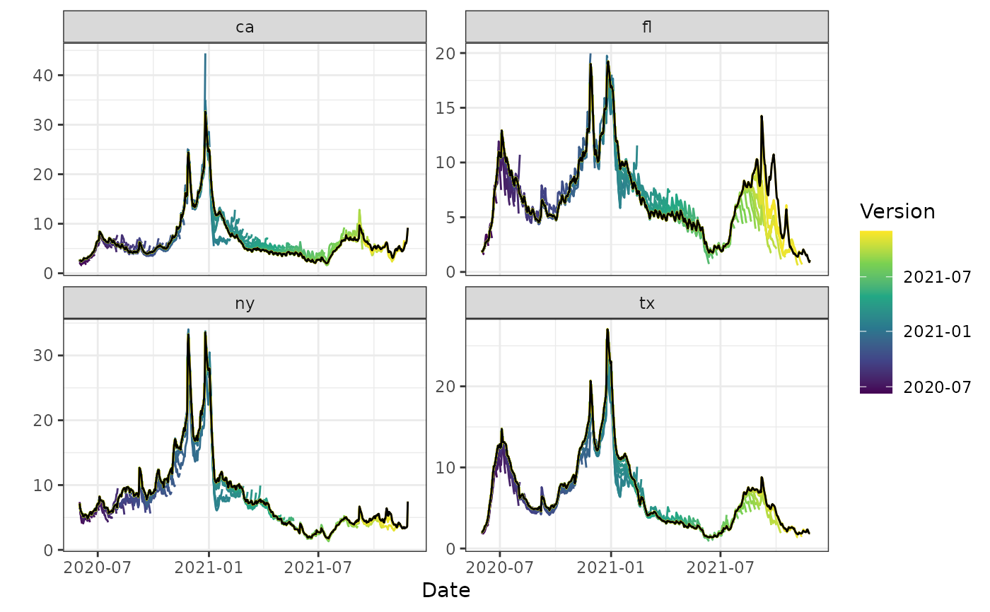
autoplot(archive_cases_dv_subset, percent_cli, .versions = "week")
#> Warning: Removed 16 rows containing missing values or values outside the scale range
#> (`geom_line()`).
# -- Use it on an archive
autoplot(archive_cases_dv_subset, percent_cli, .versions = "week")
#> Warning: Removed 16 rows containing missing values or values outside the scale range
#> (`geom_line()`).
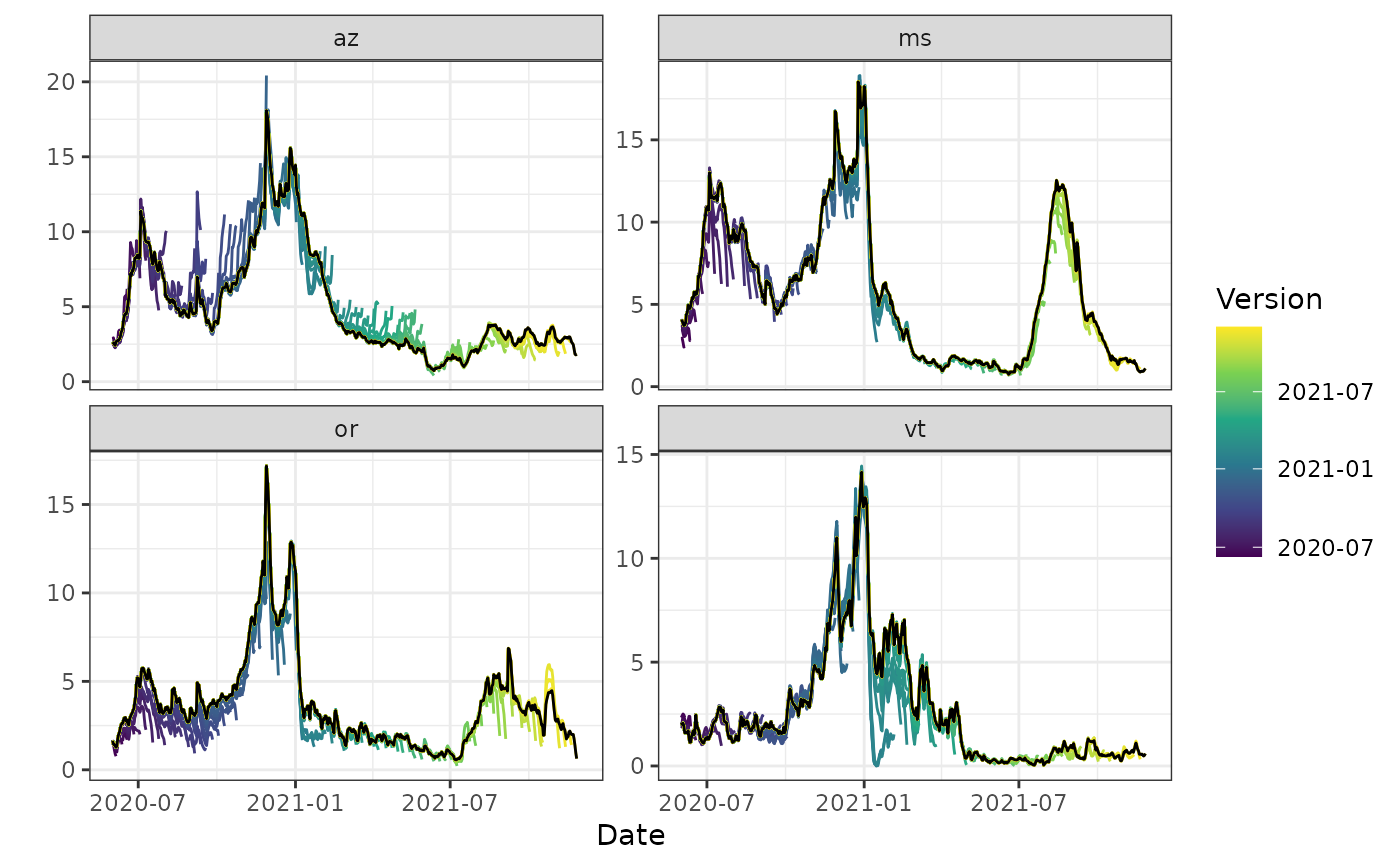
 autoplot(archive_cases_dv_subset_all_states, percent_cli,
.versions = "week",
.facet_filter = geo_value %in% c("or", "az", "vt", "ms")
)
#> Warning: Removed 16 rows containing missing values or values outside the scale range
#> (`geom_line()`).
autoplot(archive_cases_dv_subset_all_states, percent_cli,
.versions = "week",
.facet_filter = geo_value %in% c("or", "az", "vt", "ms")
)
#> Warning: Removed 16 rows containing missing values or values outside the scale range
#> (`geom_line()`).
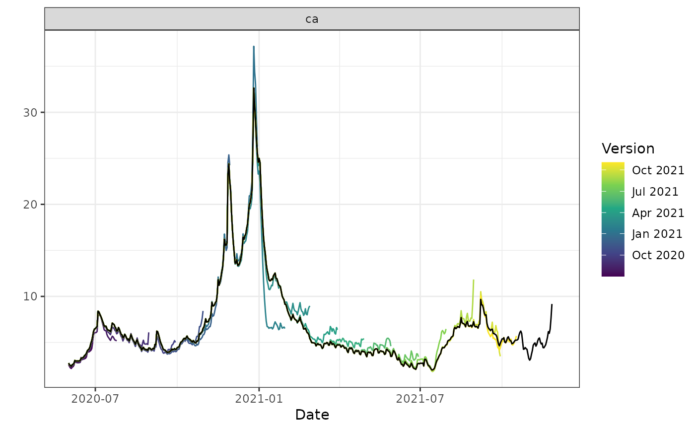
 autoplot(archive_cases_dv_subset, percent_cli,
.versions = "month",
.facet_filter = geo_value == "ca"
)
#> Warning: Removed 4 rows containing missing values or values outside the scale range
#> (`geom_line()`).
autoplot(archive_cases_dv_subset, percent_cli,
.versions = "month",
.facet_filter = geo_value == "ca"
)
#> Warning: Removed 4 rows containing missing values or values outside the scale range
#> (`geom_line()`).
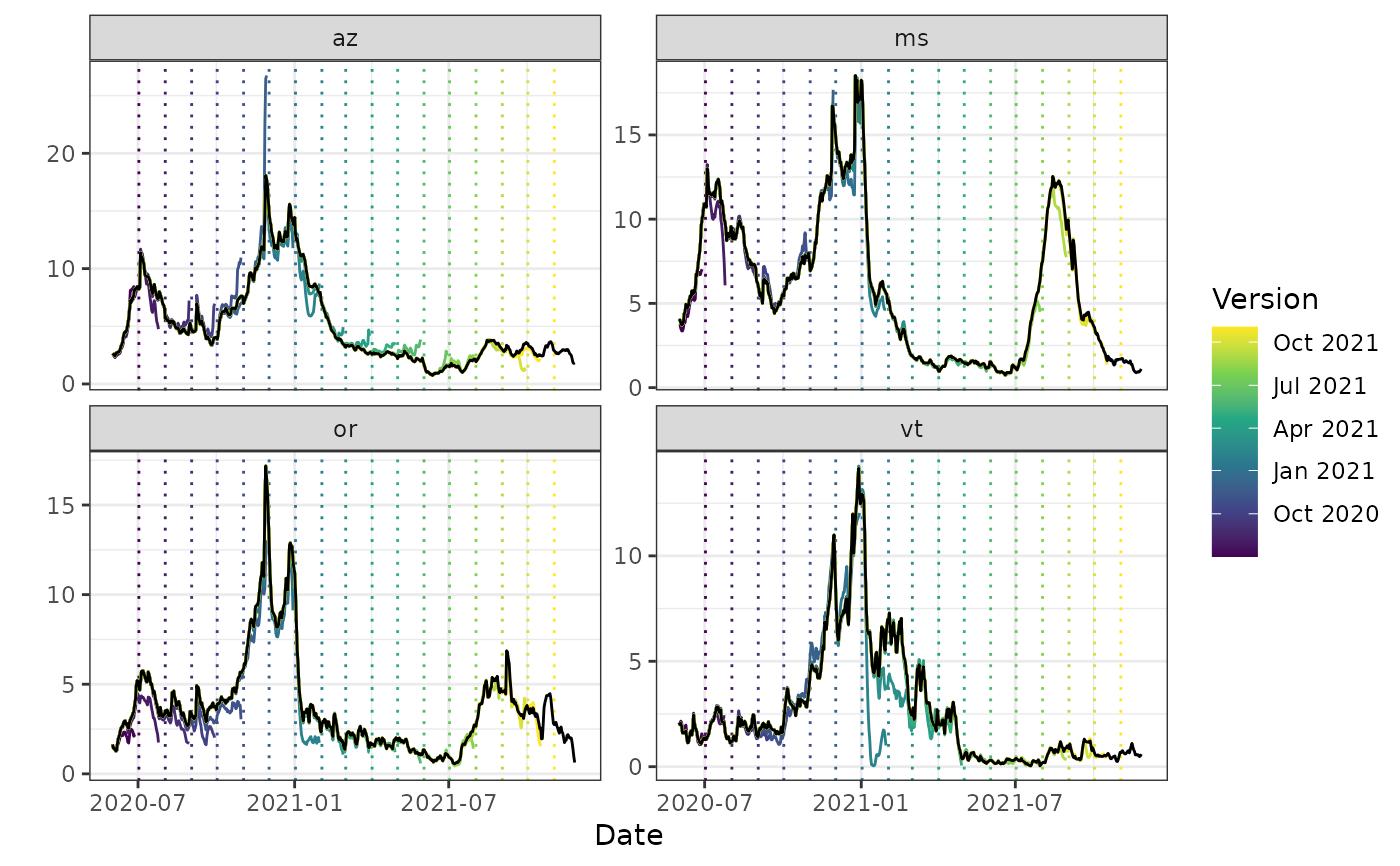
 autoplot(archive_cases_dv_subset_all_states, percent_cli,
.versions = "1 month",
.facet_filter = geo_value %in% c("or", "az", "vt", "ms"),
.mark_versions = TRUE
)
#> Warning: Removed 16 rows containing missing values or values outside the scale range
#> (`geom_line()`).
autoplot(archive_cases_dv_subset_all_states, percent_cli,
.versions = "1 month",
.facet_filter = geo_value %in% c("or", "az", "vt", "ms"),
.mark_versions = TRUE
)
#> Warning: Removed 16 rows containing missing values or values outside the scale range
#> (`geom_line()`).
 # Just an alias for convenience
plot(archive_cases_dv_subset_all_states, percent_cli,
.versions = "1 month",
.facet_filter = geo_value %in% c("or", "az", "vt", "ms"),
.mark_versions = TRUE
)
#> Warning: Removed 16 rows containing missing values or values outside the scale range
#> (`geom_line()`).
# Just an alias for convenience
plot(archive_cases_dv_subset_all_states, percent_cli,
.versions = "1 month",
.facet_filter = geo_value %in% c("or", "az", "vt", "ms"),
.mark_versions = TRUE
)
#> Warning: Removed 16 rows containing missing values or values outside the scale range
#> (`geom_line()`).