Data Cleaning, Versioning, Nowcasting With {epiprocess}
InsightNet Forecasting Workshop 2024
Alice Cima, Rachel Lobay, Daniel McDonald, Ryan Tibshirani
with huge thanks to Logan Brooks, Xueda Shen, and also to Nat DeFries, Dmitry Shemetov, and David Weber
11 December – Afternoon
Outline
Essentials of
{dplyr}and{tidyr}Epiverse Software ecosystem
Panel and Versioned Data in the epiverse
Basic Nowcasting using
{epiprocess}Nowcasting with One Variable
Nowcasting with Two Variables
Case Study - Nowcasting Cases Using %CLI
1 Essentials of {dplyr} and {tidyr}
Down with spreadsheets for data manipulation
- Spreadsheets make it difficult to rerun analyses consistently.
- Using R (and
{dplyr}) allows for:- Reproducibility
- Ease of modification
- Recommendation: Avoid manual edits; instead, use code for transformations.
- Let’s see what we mean by this…
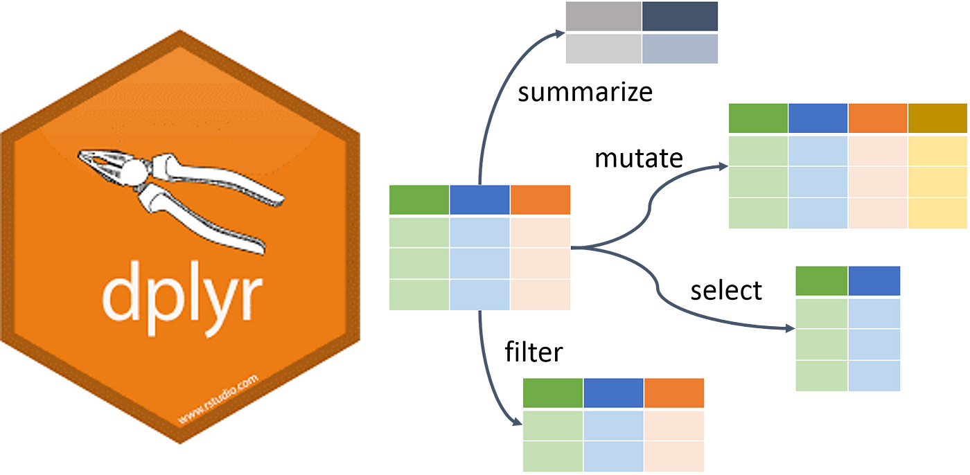
Introduction to dplyr
dplyris a powerful package in R for data manipulation.- It is part of the
tidyverse, which includes a collection of packages designed to work together… Here’s some of its greatest hits:
Introduction to dplyr
To load dplyr, you may simply load the tidyverse package:
Our focus will be on basic operations like selecting and filtering data.
Downloading JHU CSSE COVID-19 case data
- Let’s start with something familiar… Here’s a task for you:
- Use
pub_covidcast()to download JHU CSSE COVID-19 confirmed case data (confirmed_incidence_num) for CA, NC, and NY from March 1, 2022 to March 31, 2022 as of January 1, 2024. - Try this for yourself. Then click the dropdown on the next slide to check your work…
Downloading JHU CSSE COVID-19 case data
Now we only really need a few columns here…
Ways to inspect the dataset
Use head() to view the first six row of the data
# A tibble: 6 × 3
  geo_value time_value raw_cases
  <chr>     <date>         <dbl>
1 ca        2022-03-01      4310
2 nc        2022-03-01      1231
3 ny        2022-03-01      1487
4 ca        2022-03-02      7044
5 nc        2022-03-02      2243
6 ny        2022-03-02      1889
and tail to view the last six
# A tibble: 6 × 3
  geo_value time_value raw_cases
  <chr>     <date>         <dbl>
1 ca        2022-03-30      3785
2 nc        2022-03-30      1067
3 ny        2022-03-30      3127
4 ca        2022-03-31      4533
5 nc        2022-03-31      1075
6 ny        2022-03-31      4763
Selecting columns with select()
The select() function is used to pick specific columns from your dataset.
# A tibble: 93 × 2
   time_value raw_cases
   <date>         <dbl>
 1 2022-03-01      4310
 2 2022-03-01      1231
 3 2022-03-01      1487
 4 2022-03-02      7044
 5 2022-03-02      2243
 6 2022-03-02      1889
 7 2022-03-03      7509
 8 2022-03-03      2377
 9 2022-03-03      2390
10 2022-03-04      3586
# ℹ 83 more rows
Selecting columns with select()
You can exclude columns by prefixing the column names with a minus sign -.
# A tibble: 93 × 2
   time_value raw_cases
   <date>         <dbl>
 1 2022-03-01      4310
 2 2022-03-01      1231
 3 2022-03-01      1487
 4 2022-03-02      7044
 5 2022-03-02      2243
 6 2022-03-02      1889
 7 2022-03-03      7509
 8 2022-03-03      2377
 9 2022-03-03      2390
10 2022-03-04      3586
# ℹ 83 more rows
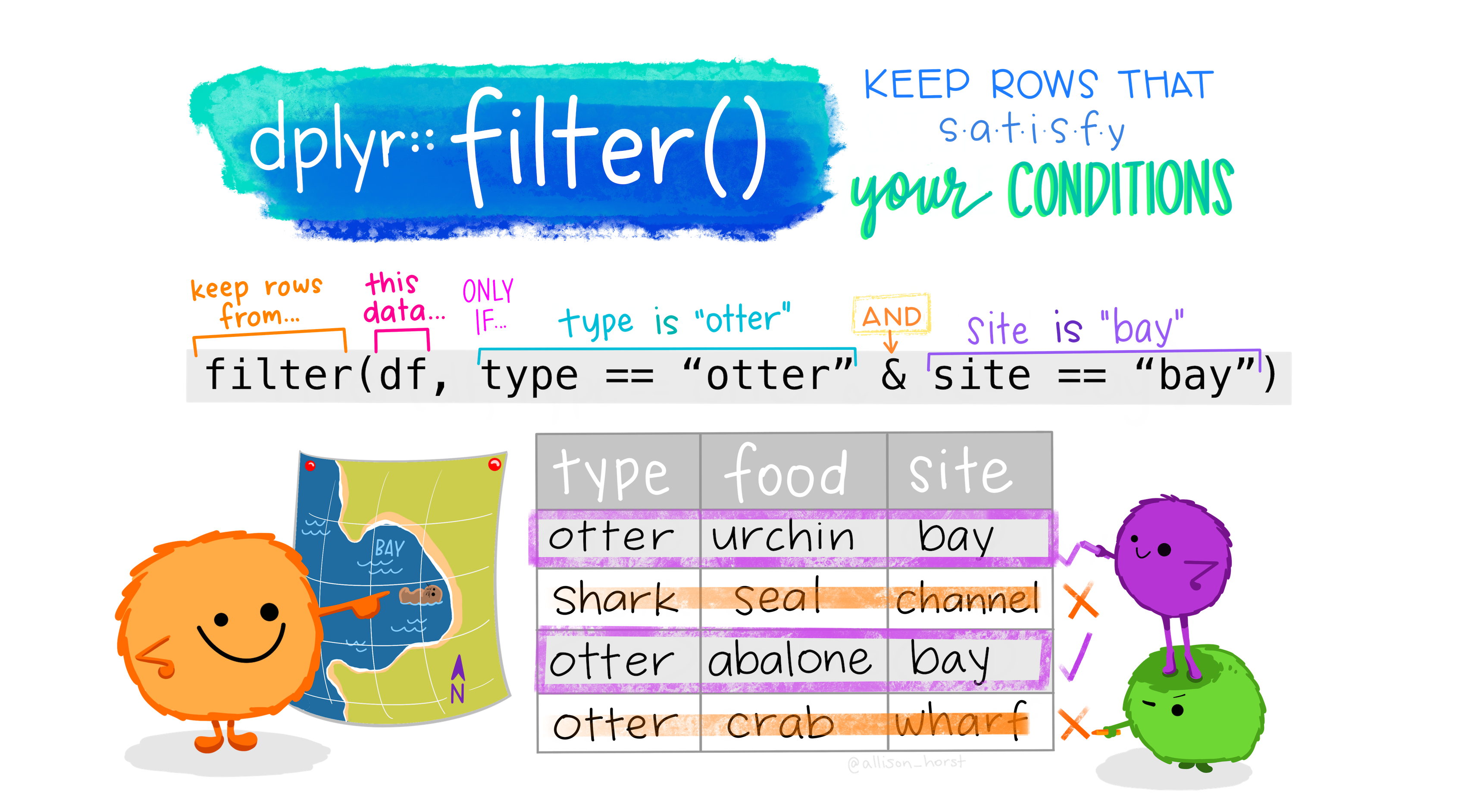
Subsetting rows with filter()
Subsetting rows with filter()
- The
filter()function allows you to subset rows that meet specific conditions. - Conditions regard column values, such as filtering for only NC or cases higher than some threshold.
- This enables you to narrow down your dataset to focus on relevant data.
# A tibble: 22 × 3
   geo_value time_value raw_cases
   <chr>     <date>         <dbl>
 1 nc        2022-03-01      1231
 2 nc        2022-03-02      2243
 3 nc        2022-03-03      2377
 4 nc        2022-03-04      2646
 5 nc        2022-03-07      4230
 6 nc        2022-03-08       894
 7 nc        2022-03-09      1833
 8 nc        2022-03-10      1783
 9 nc        2022-03-11      1849
10 nc        2022-03-14      3130
# ℹ 12 more rows
Combining select() and filter() functions
- You can further combine
select()andfilter()to further refine the dataset. - Use
select()to choose columns andfilter()to narrow down rows. - This helps in extracting the exact data needed for analysis.
Using the pipe operator |>
- The pipe operator (
|>) makes code more readable by chaining multiple operations together. - The output of one function is automatically passed to the next function.
- This allows you to perform multiple steps (e.g.,
filter()followed byselect()) in a clear and concise manner.
Grouping data with group_by()
- Use
group_by()to group data by one or more columns. - Allows performing operations on specific groups of data.
Creating new columns with mutate()
Creating new columns with mutate()
mutate()is used to create new columns.- Perform calculations using existing columns and assign to new columns.
ny_subset = cases_df |>
  filter(geo_value == "ny")

ny_subset |>
  mutate(cumulative_cases = cumsum(raw_cases)) |>
  head()
# A tibble: 6 × 4
geo_value time_value raw_cases cumulative_cases
<chr> <date> <dbl> <dbl>
1 ny 2022-03-01 1487 1487
2 ny 2022-03-02 1889 3376
3 ny 2022-03-03 2390 5766
4 ny 2022-03-04 350 6116
5 ny 2022-03-05 3372 9488
6 ny 2022-03-06 2343 11831Combining group_by() and mutate()
- First, group data using
group_by(). - Then, use
mutateto perform the calculations for each group. - Finally, use
arrangeto display the output bygeo_value.
cases_df |>
  group_by(geo_value) |>
  mutate(cumulative_cases = cumsum(raw_cases)) |>
  arrange(geo_value) |>
  head()
# A tibble: 6 × 4
# Groups: geo_value [1]
geo_value time_value raw_cases cumulative_cases
<chr> <date> <dbl> <dbl>
1 ca 2022-03-01 4310 4310
2 ca 2022-03-02 7044 11354
3 ca 2022-03-03 7509 18863
4 ca 2022-03-04 3586 22449
5 ca 2022-03-05 1438 23887
6 ca 2022-03-06 6465 30352Summarizing data with summarise()
summarise()reduces data to summary statistics (e.g., mean, median).- Typically used after
group_by()to summarize each group.
Key practices learned
- Use
head()andtail()for quick data inspection. - Use
select()andfilter()for data manipulation. - Chain functions with
|>. - Use
group_by()to group data by one or more variables before applying functions. - Use
mutateto create new columns or modify existing ones by applying functions to existing data. - Use
summariseto reduce data to summary statistics (e.g., mean, median).
1 to 2 word summaries of the dplyr functions
Here are 1 to 2 word summaries of the key dplyr functions:
select(): Choose columnsfilter(): Subset rowsmutate(): Create columnsgroup_by(): Group bysummarise(): Numerical summary
Tidy data and Tolstoy
“Happy families are all alike; every unhappy family is unhappy in its own way.” — Leo Tolstoy

What is tidy data?
- Tidy data follows a consistent structure: each row represents one observation, and each column represents one variable.
cases_dfis one classic example of tidy data.
# A tibble: 6 × 3
  geo_value time_value raw_cases
  <chr>     <date>         <dbl>
1 ca        2022-03-01      4310
2 nc        2022-03-01      1231
3 ny        2022-03-01      1487
4 ca        2022-03-02      7044
5 nc        2022-03-02      2243
6 ny 2022-03-02 1889- To convert between tidy and messy data, we can use the
tidyrpackage in the tidyverse.
pivot_wider() and pivot_longer()
Making data wider with pivot_wider()
- To convert data from long format to wide/messy format use
pivot_wider(). - For example, let’s try creating a column for each time value in
cases_df:
messy_cases_df <- cases_df |>
  pivot_wider(
    names_from = time_value,   # Create new columns for each unique date
    values_from = raw_cases    # Fill those columns with the raw_case values
  )

# View the result
messy_cases_df
# A tibble: 3 × 32
geo_value `2022-03-01` `2022-03-02` `2022-03-03` `2022-03-04` `2022-03-05`
<chr> <dbl> <dbl> <dbl> <dbl> <dbl>
1 ca 4310 7044 7509 3586 1438
2 nc 1231 2243 2377 2646 0
3 ny 1487 1889 2390 350 3372
# ℹ 26 more variables: `2022-03-06` <dbl>, `2022-03-07` <dbl>,
# `2022-03-08` <dbl>, `2022-03-09` <dbl>, `2022-03-10` <dbl>,
# `2022-03-11` <dbl>, `2022-03-12` <dbl>, `2022-03-13` <dbl>,
# `2022-03-14` <dbl>, `2022-03-15` <dbl>, `2022-03-16` <dbl>,
# `2022-03-17` <dbl>, `2022-03-18` <dbl>, `2022-03-19` <dbl>,
# `2022-03-20` <dbl>, `2022-03-21` <dbl>, `2022-03-22` <dbl>,
# `2022-03-23` <dbl>, `2022-03-24` <dbl>, `2022-03-25` <dbl>, …Tidying messy data with pivot_longer()
- Use
pivot_longer()to convert data from wide format (multiple columns for the same variable) to long format (one column per variable). - Let’s try turning
messy_cases_dfback into the original tidycases_df!
tidy_cases_df <- messy_cases_df |>
  pivot_longer(
    cols = -geo_value,          # Keep the 'geo_value' column as it is
    names_to = "time_value",    # Create a new 'time_value' column from the column names
    values_to = "raw_cases"     # Values from the wide columns should go into 'raw_cases'
  )

# View the result
head(tidy_cases_df, n = 3) # Notice the class of time_value here
# A tibble: 3 × 3
geo_value time_value raw_cases
<chr> <chr> <dbl>
1 ca 2022-03-01 4310
2 ca 2022-03-02 7044
3 ca 2022-03-03 7509Introduction to joins in dplyr
- Joining datasets is a powerful tool for combining info. from multiple sources.
- In R,
dplyrprovides several functions to perform different types of joins. - We’ll demonstrate joining a subset of
cases_df(our case counts dataset) withstate_census. - Motivation: We can scale the case counts by population to make them comparable across regions of different sizes.
Subset cases_df
To simplify things, let’s use filter() to only grab one date of cases_df:
# A tibble: 3 × 3
  geo_value time_value raw_cases
  <chr>     <date>         <dbl>
1 ca        2022-03-01      4310
2 nc        2022-03-01      1231
3 ny        2022-03-01      1487
Though note that what we’re going to do can be applied to the entirety of cases_df.
Load state census data
The state_census dataset from epidatasets contains state populations from the 2019 census.
# State census dataset from epidatasets
library(epidatasets)
state_census = state_census |> select(abbr, pop) |> filter(abbr != "us")

state_census |> head()
# A tibble: 6 × 2
abbr pop
<chr> <dbl>
1 al 4903185
2 ak 731545
3 az 7278717
4 ar 3017804
5 ca 39512223
6 co 5758736Notice that this includes many states that are not in cases_df_sub.
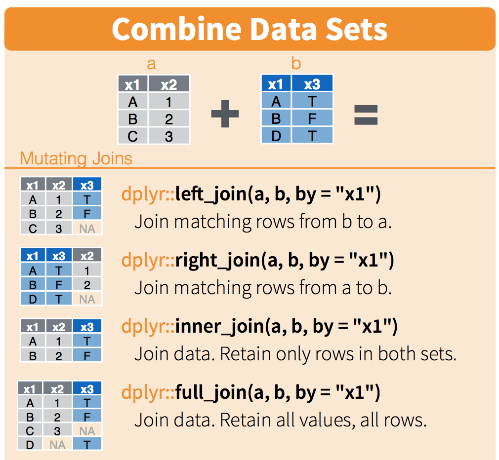
Left Join: Keep all rows from the first dataset
- A left join keeps all rows from the first dataset (
cases_df_sub), and adds matching data from the second dataset (state_census). - So all rows from the first dataset (
cases_df_sub) will be preserved. - The datasets are joined by matching the
geo_valuecolumn, specified by the by argument.
# Left join: combining March 1, 2022 state case data with the census data
cases_sub_left_join <- cases_df_sub |>
  left_join(state_census, join_by(geo_value == abbr))

cases_sub_left_join
# A tibble: 3 × 4
geo_value time_value raw_cases pop
<chr> <date> <dbl> <dbl>
1 ca 2022-03-01 4310 39512223
2 nc 2022-03-01 1231 10488084
3 ny 2022-03-01 1487 19453561Right Join: Keep all rows from the second dataset
- A right join keeps all rows from the second dataset (
state_census), and adds matching data from the first dataset (cases_df_sub). - If a row in the second dataset doesn’t have a match in the first, then the columns from the first will be filled with NA.
- For example, can see this for the
alrow fromstate_census…
# Right join: keep all rows from state_census
cases_sub_right_join <- cases_df_sub |>
  right_join(state_census, join_by(geo_value == abbr))

head(cases_sub_right_join)
# A tibble: 6 × 4
geo_value time_value raw_cases pop
<chr> <date> <dbl> <dbl>
1 ca 2022-03-01 4310 39512223
2 nc 2022-03-01 1231 10488084
3 ny 2022-03-01 1487 19453561
4 al NA NA 4903185
5 ak NA NA 731545
6 az NA NA 7278717Inner Join: Only keep matching rows
- An inner join will only keep rows where there is a match in both datasets.
- So, if a state in
state_censusdoes not have a corresponding entry incases_df_sub, then that row will be excluded.
# Inner join: only matching rows are kept
cases_sub_inner_join <- cases_df_sub |>
  inner_join(state_census, join_by(geo_value == abbr))

cases_sub_inner_join
# A tibble: 3 × 4
geo_value time_value raw_cases pop
<chr> <date> <dbl> <dbl>
1 ca 2022-03-01 4310 39512223
2 nc 2022-03-01 1231 10488084
3 ny 2022-03-01 1487 19453561Full Join: Keep all rows from both datasets
- A full join will keep all rows from both datasets.
- If a state in either dataset has no match in the other, the missing values will be filled with NA.
# Full join: keep all rows from both datasets
cases_sub_full_join <- cases_df_sub |>
  full_join(state_census, join_by(geo_value == abbr))

head(cases_sub_full_join)
# A tibble: 6 × 4
geo_value time_value raw_cases pop
<chr> <date> <dbl> <dbl>
1 ca 2022-03-01 4310 39512223
2 nc 2022-03-01 1231 10488084
3 ny 2022-03-01 1487 19453561
4 al NA NA 4903185
5 ak NA NA 731545
6 az NA NA 7278717Pictorial summary of the four join functions
Two review questions
Q1): What join function should you use if your goal is to scale the cases by population in cases_df?
Q2): Lastly, please create a new column in cases_df where you scale the cases by population and multiply by 1e5 to get cases / 100k.
Congratulations for making it through this crash course! That’s all for this glimpse() into the tidyverse.
2 Epiverse Software Ecosystem
Epi. data processing with epiprocess
epiprocessis a package that offers additional functionality to pre-process epidemiological data.- You can work with an
epi_dflike you can with a tibble by using dplyr verbs. - For example, on
cases_df, we can easily useepi_slide_mean()to calculate trailing 14 day averages of cases:
An `epi_df` object, 93 x 6 with metadata:
* geo_type  = state
* time_type = day
* as_of     = 2024-01-01

# A tibble: 93 × 6
# Groups:   geo_value [3]
   geo_value time_value raw_cases      pop scaled_cases smoothed_scaled_cases
 * <chr>     <date>         <dbl>    <dbl>        <dbl>                 <dbl>
 1 ca        2022-03-01      4310 39512223        10.9                   10.9
 2 ca        2022-03-02      7044 39512223        17.8                   14.4
 3 ca        2022-03-03      7509 39512223        19.0                   15.9
 4 ca        2022-03-04      3586 39512223         9.08                  14.2
 5 ca        2022-03-05      1438 39512223         3.64                  12.1
 6 ca        2022-03-06      6465 39512223        16.4                   12.8
 7 ca        2022-03-07      6690 39512223        16.9                   13.4
 8 ca        2022-03-08      3424 39512223         8.67                  12.8
 9 ca        2022-03-09      4591 39512223        11.6                   12.7
10 ca        2022-03-10      5359 39512223        13.6                   12.8
# ℹ 83 more rows
Epi. data processing with epiprocess
It is easy to produce an autoplot of the smoothed confirmed daily cases for each geo_value:
Epi. data processing with epiprocess
Alternatively, we can display both the smoothed and the original daily case rates:
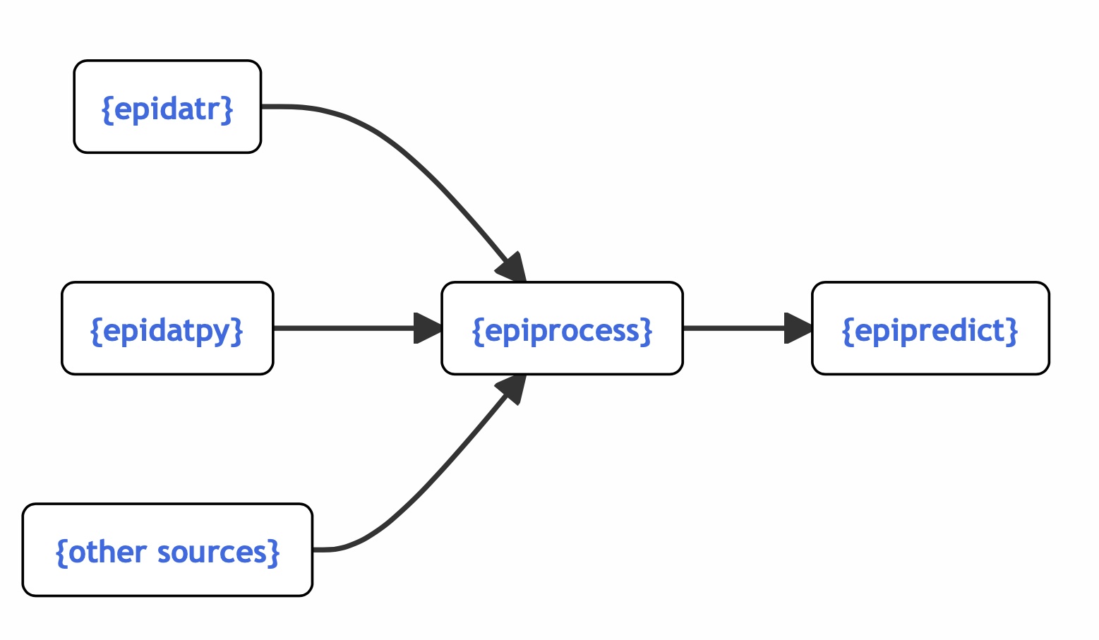
Now, before exploring some more features of epiprocess, let’s have a look at the epiverse software ecosystem it’s part of…
The epiverse ecosystem
Interworking, community-driven, packages for epi tracking & forecasting.
3 Panel and Versioned Data in the Epiverse
What is panel data?
- Recall that panel data, or longitudinal data, contain cross-sectional measurements of subjects over time.
- Built-in example:
covid_case_death_ratesdataset, which is a snapshot as of May 31, 2022 that contains daily state-wise measures ofcase_rateanddeath_ratefor COVID-19 over 2021:
# A tibble: 6 × 4
  geo_value time_value case_rate death_rate
  <chr>     <date>         <dbl>      <dbl>
1 ak        2020-12-31      35.9      0.158
2 al        2020-12-31      65.1      0.438
3 ar        2020-12-31      66.0      1.27
4 az        2020-12-31      76.8      1.10
5 ca        2020-12-31      96.0      0.751
6 co 2020-12-31 35.8 0.649- How do we store & work with such snapshots in the epiverse software ecosystem?
epi_df: Snapshot of a dataset
- You can convert panel data into an
epi_dfwith the requiredgeo_valueandtime_valuecolumns
Therefore, an epi_df is…
a tibble that requires columns
geo_valueandtime_value.arbitrary additional columns containing measured values
additional keys to index (
age_group,ethnicity, etc.)
epi_df
Represents a snapshot that contains the most up-to-date values of the signal variables, as of a given time.
epi_df: Snapshot of a dataset
Consider the same dataset we just encountered on JHU daily COVID-19 cases and deaths rates from all states as of May 31, 2022.
We can see that it meets the criteria
epi_df(hasgeo_valueandtime_valuecolumns) and that it contains additional metadata (i.e.geo_type,time_type,as_of, andother_keys).
An `epi_df` object, 6 x 4 with metadata:
* geo_type  = state
* time_type = day
* as_of     = 2022-05-31

# A tibble: 6 × 4
  geo_value time_value case_rate death_rate
* <chr>     <date>         <dbl>      <dbl>
1 ak        2020-12-31      35.9      0.158
2 al        2020-12-31      65.1      0.438
3 ar        2020-12-31      66.0      1.27
4 az        2020-12-31      76.8      1.10
5 ca        2020-12-31      96.0      0.751
6 co 2020-12-31 35.8 0.649Examples of preprocessing
EDA features
- Making locations commensurate (per capita scaling)
- Correlating signals across location or time
- Computing growth rates
- Detecting and removing outliers
- Calculating summaries with rolling windows
- Dealing with revisions
Features - Correlations at different lags
The below plot addresses the question: “For each state, are case and death rates linearly associated across all days?”
To explore lagged correlations and how case rates associate with future death rates, we can use the
dt1parameter inepi_cor()to shift case rates by a specified number of days.
- We can see that, in general, lagging the case rates back by 14 days improves the correlations.
Features - Systematic lag analysis
The analysis helps identify the lag at which case rates from the past have the strongest correlation with future death rates.
The strongest correlation occurs at a lag of about 23 days, indicating that case rates are best correlated with death rates 23 days from now.
Features - Compute growth rates
Growth rate measures the relative change in a signal over time.
We can compute time-varying growth rates for the two states, and see how this cases evolves over time.
- As expected, the peak growth rates for both states occurred during the January 2022 Omicron wave, reflecting the sharp rise in cases over that period.
Features - Outlier detection
The
detect_outlr()function offers multiple outlier detection methods on a signal.The simplest is
detect_outlr_rm(), which works by calculating an outlier threshold using the rolling median and the rolling Interquartile Range (IQR) for each time point:
Threshold = Rolling Median ± (Detection Multiplier × Rolling IQR)
- Note that the default number of time steps to use in the rolling window by default is 21 and is centrally aligned.
- The detection multiplier default is 2 and controls how far away a data point must be from the median to be considered an outlier.
Features - Outlier detection
Several data points that deviate from the expected case cadence have been flagged as outliers, and may require further investigation.
However, the peak in Jan. 2022 has also been flagged as an outlier. This highlights the importance of manual inspection before correcting the data, as these may represent valid events (e.g., a genuine surge in cases).
Features – sliding a computation on an epi_df
It is often useful to compute rolling summaries of signals.
These depend on the reference time, and are computed separately over geographies (and other groups).
For example, a trailing average can smooth out daily variation.
In
epiprocess, this is achieved byepi_slide().
For example, we can use epi_slide() to compute a trailing 7-day average.
Features – sliding a computation on an epi_df
The simplest way to use
epi_slideis tidy evaluation.For a grouped
epi_df,epi_slide()applies the computation to groups separately.
# A tibble: 6 × 4
  geo_value time_value raw_cases cases_7dav
  <chr>     <date>         <dbl>      <dbl>
1 ca        2022-03-01      4310       4310
2 ca        2022-03-02      7044       5677
3 nc        2022-03-01      1231       1231
4 nc        2022-03-02      2243       1737
5 ny        2022-03-01      1487       1487
6 ny        2022-03-02      1889       1688
Features – sliding a computation on an epi_df
epi_slide also accepts custom functions of a certain form.
x: the data frame with all the columns with original object except groupping vars.g: the one-row tibble with values of gropping vars of the given group.t: the.ref_time_valueof the current window....: additional arguments.
Features – sliding a computation on an epi_df
# A tibble: 3 × 4
  geo_value time_value raw_cases cases_7dav
  <chr>     <date>         <dbl>      <dbl>
1 ca        2022-03-01      4310       4310
2 nc        2022-03-01      1231       1231
3 ny 2022-03-01 1487 1487epi_archive: Collection of epi_dfs
- full version history of a data set
- acts like a bunch of
epi_dfs — but stored compactly - allows similar functionality as
epi_dfbut using only data that would have been available at the time
Revisions
Epidemiology data gets revised frequently.
- We may want to use the data [as it looked in the past].{.primary}
- or we may want to examine the history of revisions.
epi_archive: Collection of epi_dfs
Subset of daily COVID-19 doctor visits (Optum) and cases (JHU CSSE) from all U.S. states in archive format:
$DT
Key: <geo_value, time_value, version>
         geo_value time_value    version percent_cli case_rate_7d_av
            <char>     <Date>     <Date>       <num>           <num>
      1:        ak 2020-06-01 2020-06-02          NA        1.145652
      2:        ak 2020-06-01 2020-06-06    0.136815        1.145652
      3:        ak 2020-06-01 2020-06-08    0.136249        1.145652
      4:        ak 2020-06-01 2020-06-09    0.106744        1.145652
      5:        ak 2020-06-01 2020-06-10    0.106676        1.145652
     ---
1514485:        wy 2021-11-26 2021-11-29    3.739819       23.207343
1514486:        wy 2021-11-27 2021-11-28          NA       23.207343
1514487:        wy 2021-11-28 2021-11-29          NA       23.207343
1514488:        wy 2021-11-29 2021-11-30          NA       25.071781
1514489:        wy 2021-11-30 2021-12-01          NA       25.464294

$geo_type
[1] "state"

$time_type
[1] "day"

$other_keys
character(0)

$clobberable_versions_start
[1] NA

$versions_end
[1] "2021-12-01"
Features – sliding computation over epi_dfs
- We can apply a computation over different snapshots in an
epi_archive.
This functionality is very helpful in version aware forecasting. We will return with a concrete example.
Features – summarize revision behavior
revision_summary()is a helper function that summarizes revision behavior of anepix_archive.
revision_data <- revision_summary(
  archive_cases_dv_subset,
  case_rate_7d_av,
  drop_nas = TRUE,
  print_inform = FALSE, # NOT the default, to save space
  min_waiting_period = as.difftime(60, units = "days"),
  within_latest = 0.2,
  quick_revision = as.difftime(3, units = "days"),
  few_revisions = 3,
  abs_spread_threshold = NULL,
  rel_spread_threshold = 0.1,
  compactify_tol = .Machine$double.eps^0.5,
  should_compactify = TRUE
)
Features – summarize revision behavior
# A tibble: 6 × 11
  time_value geo_value n_revisions min_lag max_lag  time_near_latest spread
  <date>     <chr>           <dbl> <drtn>  <drtn>   <drtn>            <dbl>
1 2020-06-01 ca                 12 1 days  546 days 1 days           0.248
2 2020-06-02 ca                 12 1 days  545 days 1 days           0.416
3 2020-06-03 ca                 11 1 days  544 days 1 days           0.115
4 2020-06-04 ca                 11 1 days  543 days 1 days           0.342
5 2020-06-05 ca                  7 1 days  520 days 1 days           0.0982
6 2020-06-06 ca                  8 1 days  519 days 1 days           0.188
# ℹ 4 more variables: rel_spread <dbl>, min_value <dbl>, max_value <dbl>,
#   median_value <dbl>
Visualize revision patterns
Finalized data
Counts are revised as time proceeds
Want to know the final value
Often not available until weeks/months later
- Forecasting
- At time \(t\), predict the final value for time \(t+h\), \(h > 0\)
- Backcasting
- At time \(t\), predict the final value for time \(t-h\), \(h < 0\)
- Nowcasting
- At time \(t\), predict the final value for time \(t\)
4 Basic Nowcasting in the Epiverse
Backfill Canadian edition
Every week the BC CDC releases COVID-19 hospitalization data.
Following week they revise the number upward (by ~25%) due to lagged reports.
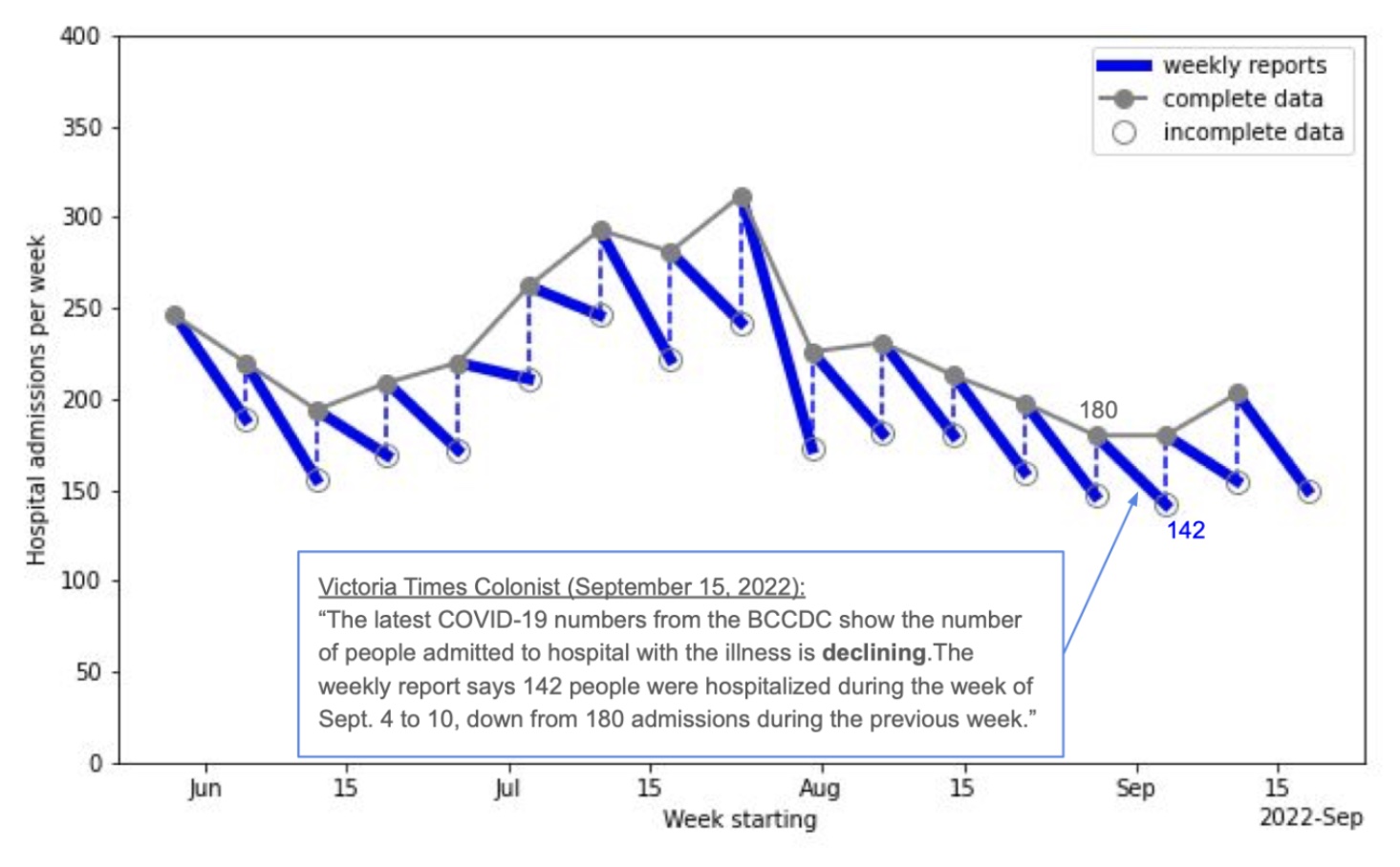
- Takeaway: Once the data is backfilled, hospitalizations rarely show a decline, challenging the common media narrative.
Backfill American edition
Again, we can see a similar systematic underestimation problem for COVID-19 mortality rates in CA.
This plot also illustrates the revision process - how the reported mortality changes & increases across multiple updates until it stabilizes at the final value (black line).
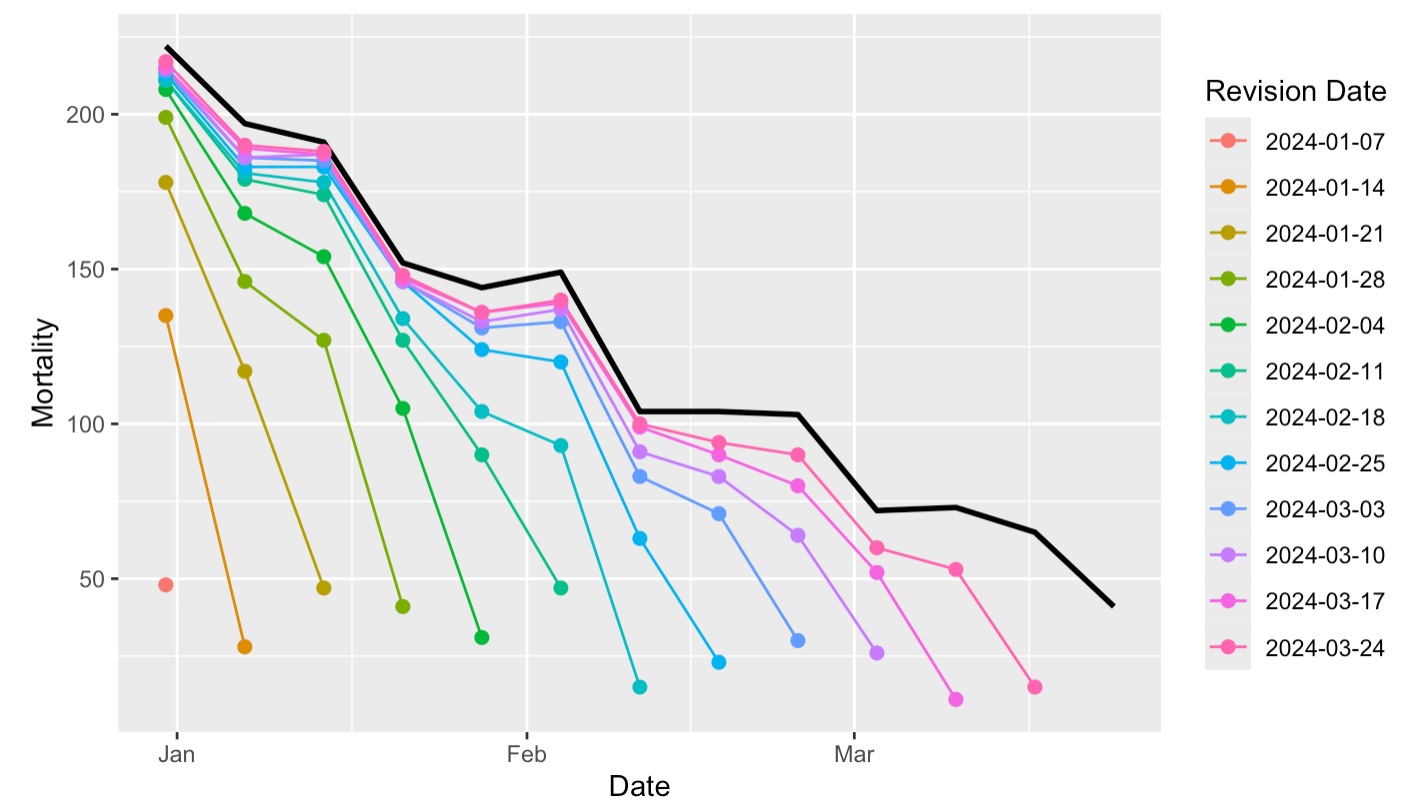
- These two examples show the problem and now we need a solution…
Nowcasting and its mathematical setup
Nowcasting: Predict a finalized value from a provisional value.
Suppose today is time \(t\)
Let \(y_i\) denote a series of interest observed at times \(i=1,\ldots, t\).
Our goal
- Produce a point nowcast for the finalized values of \(y_t\).
- Accompany with time-varying prediction intervals
- We may also have access to \(p\) other time series \(x_{ij},\; i=1,\ldots,t, \; j = 1,\ldots, p\) which may be subject to revisions.
Case study: NCHS mortality
- In this example, we’ll demonstrate the concept of nowcasting using NHCS mortality data. (the number of weekly new deaths with confirmed or presumed COVID-19, per 100,000 population).
- We will work with provisional data (real-time reports) and compare them to finalized data (final reports).
- The goal is to estimate or nowcast the mortality rate for weeks when only provisional data is available.
Fetch versioned data
Let’s fetch versioned mortality data from the API (pub_covidcast) for CA (geo_values = "ca") and the signal of interest (deaths_covid_incidence_num) over early 2024.
# Fetch the versioned NCHS mortality data (weekly)
nchs_archive <- pub_covidcast(
  source = "nchs-mortality",
  signals = "deaths_covid_incidence_num",
  geo_type = "state",
  time_type = "week",
  geo_values = c("ca", "ut"),
  time_values = epirange(202001, 202440),
  issues = "*"
) |>
  select(geo_value, time_value, version = issue, mortality = value) |>
  as_epi_archive(compactify = TRUE)
Analysis of versioning behavior
Recall, we need to watch out for:
- Latency the time difference between date of reference and date of the initial report
- Backfill how data for a given date is updated after initial report.
revision_summary() provides a summary of both aspects.
Versioning analysis – latency
- Question: What is the latency of NCHS data?
# A tibble: 10 × 3
   geo_value time_value min_lag
   <chr>     <date>     <drtn>
 1 ca        2020-07-12 147 days
 2 ca        2021-08-29  14 days
 3 ut        2020-09-27  70 days
 4 ut        2022-01-30   7 days
 5 ca        2023-07-09   7 days
 6 ut        2022-01-02   7 days
 7 ca        2023-02-12   7 days
 8 ca        2022-01-02   7 days
 9 ut        2024-04-07   7 days
10 ca 2024-09-22 7 days- We randomly sampled some dates to check if there is a consistent latency pattern.
- Understanding latency prevents us from using data that we shouldn’t have access to.
Versioning analysis – backfill
- Question: How long does it take for the reported value to be close to the finalized value?
# A tibble: 10 × 3
   geo_value time_value time_near_latest
   <chr>     <date>     <drtn>
 1 ut        2023-05-28   7 days
 2 ca        2021-08-15  28 days
 3 ut        2020-03-08 273 days
 4 ut        2021-07-25  28 days
 5 ca        2020-05-24 196 days
 6 ca        2020-06-21 168 days
 7 ca        2020-01-26 315 days
 8 ca        2020-07-19 140 days
 9 ca        2023-10-15  21 days
10 ca 2020-11-01 35 days - It generally takes at least 4 weeks for reported value to be within 20% (default in
revision_summary()) of the finalized value. - We can change the threshold of percentage difference by specifying the
within_latestargument ofrevision_summary().
Versioning analysis - backfill
- Question: When is the finalized value first attained for each date? Would we have access to any in real-time?
- How fast are the final values attained & what’s the pattern for these times, if any?
# A tibble: 6 × 4
  geo_value time_value min_version time_to_final
  <chr>     <date>     <date>      <drtn>
1 ca        2020-01-26 2020-12-06  315 days
2 ca        2020-02-09 2020-12-06  301 days
3 ca        2020-02-23 2020-12-06  287 days
4 ca        2020-03-15 2020-12-06  266 days
5 ca        2020-03-22 2021-05-16  420 days
6 ca 2020-03-29 2021-04-04 371 days - Conclusion: The revision behavior is pretty long-tailed. Value reported 4 weeks later is reasonably close to the finalized value.
Revision pattern visualization
This shows the finalized rates in comparison to multiple revisions to see how the data changes over time:
Revision pattern visualization
Ratio nowcaster: jumping from provisional to finalized value
- Recall, the goal of nowcast at date \(t\) is to use project the finalized value of \(y_t,\) given the information available on date \(t\).
- A very simple nowcaster is the ratio between finalized and provisional value.
How can we sensibly estimate this quantity?
Ratio nowcaster: building training samples
- At nowcast date \(t,\) would have received reports with versions up to and including \(t.\)
- We need to build training samples, which
- correctly aligns finalized value against provisional value
- uses features that would have been available at test time
- have enough samples to ensure sensible estimation results
- Build training samples by treating dates prior to date \(t\) as actual nowcast dates.
- What is the provisional data on that date?
- Have we received finalized value for that date?
Ratio nowcaster: building training samples
- At an earlier nowcast date \(t_0,\) we define
- Provisional value as the reported value of \(Y_{s_0}\) with version \(t_0.\) Here \(s_0\) is the largest occurence date among all values reported up until \(t_0.\)
- Finalized value as the (potentially unobserved) finalized value of \(Y_{s_0}.\)
- We only know in hindsight when reported value of \(Y_{s_0}\) is finalized – need an approximation.
Revisiting revision_summary()
Recall, revision_summary() reports the number of days to be within 20% (default value) of finalized value
# A tibble: 5 × 3
  geo_value time_value time_near_latest
  <chr>     <date>     <drtn>
1 ut        2023-04-09  7 days
2 ut        2022-03-06 49 days
3 ca        2021-01-24 49 days
4 ut        2020-09-20 77 days
5 ca        2021-01-17 49 days
Time differences in days
0% 25% 50% 75% 100%
7 21 28 49 315 Let’s say data reported 49 days after reference date is good enough to be considered finalized.
Ratio nowcaster: test time feature
- Due to latency, provisional values may not be available at lag 0
- We use last-observation-carried-forward (LOCF) to impute missing values at test time
- Precisely, at test time \(t,\) we use last observed data point (among all those reported up through time \(t\))
Nowcasting at a single date: building training samples
- Searching for provisional values, at previous hypothetical nowcast dates.
- Searching for finalized values, at previous hypothetical nowcast dates.
Nowcasting at a single date: estimating ratio model
- After searching for both provisional and finalized values, we merge them together and estimate the ratio.
Nowcasting at a single date: test feature construction
Nowcasting at a single date: producing the nowcast
nowcast <- last_avail * ratio
finalized_val <- epix_as_of(nchs_archive, nchs_archive$versions_end) |>
filter(time_value == nowcast_date) |>
pull(mortality)
nowcast_final = data.frame(Nowcast = nowcast, `Finalized value` = finalized_val, check.names=FALSE)
knitr::kable(nowcast_final)| Nowcast | Finalized value |
|---|---|
| 305.1608 | 946 |
Nowcasting for multiple dates
- All previous manipulations should really be seen as a template for all nowcast dates.
- The template computation sould be applied over all nowcast dates, but we must respect data versioning!
epix_slide()is designed just for this! It behaves similarly toepi_slide.- Key exception:
epix_slide()is version aware: the sliding computation at any reference time \(t\) is performed on data that would have been available as of t.
Nowcasting for multiple dates via epix_slide()
We begin by templatizing our previous operations.
nowcaster <- function(x, g, t, wl=180, appx=approx_final_lag) {
initial_data <- x$DT |>
group_by(geo_value, time_value) |>
filter(version == min(version)) |>
filter(time_value >= t - wl - appx & time_value <= t - appx) |>
rename(initial_val = mortality) |>
select(geo_value, time_value, initial_val)
finalized_data <- x$DT |>
group_by(geo_value, time_value) |>
filter(version == max(version)) |>
filter(time_value >= t - wl - appx & time_value <= t - appx) |>
rename(finalized_val = mortality) |>
select(geo_value, time_value, finalized_val)
ratio <- finalized_data |>
  inner_join(initial_data, by = c("geo_value", "time_value")) |>
  mutate(ratio = finalized_val / initial_val) |>
  pull(ratio) |>
  median(na.rm = TRUE)
last_avail <- epix_as_of(x, t) |>
slice_max(time_value) |>
pull(mortality)
tibble(geo_value = x$geo_value, target_date = t, nowcast = last_avail * ratio)
}Sanity check of epix_slide()
slided_nowcast_1d = epix_slide(
  .x = nchs_archive,
  .f = nowcaster,
  .before = Inf,
  .versions = nowcast_date,
  .all_versions = TRUE
)

nowcast_check = data.frame(`Manual nowcast` = nowcast, `Slided nowcast` = slided_nowcast_1d$nowcast, check.names = FALSE)
knitr::kable(nowcast_check)| Manual nowcast | Slided nowcast |
|---|---|
| 305.1608 | 305.1608 |
Nowcasting for multiple dates via epix_slide()
Details of epix_slide()
.finepix_slide()can be specified with the same form of custom function asepi_slide().
- Mandatory variables of
.fwould have different forms depending on the value of.all_versions.
Details of epix_slide()
- When
.all_versions = FALSE,epix_slide()essentially iterates the templatized computation over snapshots. - Said differently, when
.all_versions = FALSE, data accessed at any sliding iteration only involves a single version.
- Hence:
x: anepi_dfwith same column names as archive’sDT, minus theversioncolumn.g: a one-row tibble containing the values of groupping variables of the associated group.t: theref_time_valueof the current window....: additional arguments.
Details of epix_slide()
- When
.all_versions = FALSE, data accessed at any sliding iteration involves versions up to and including .version.
- Hence:
x: anepi_archive, with version up to and including.version.g: a one-row tibble containing the values of groupping variables of the associated group.t: the.versionof the current window....: additional arguments.
Details of epix_slide()
Details of epix_slide()
nowcaster <- function(x, g, t, wl=180, appx=approx_final_lag) {
  initial_data <- x$DT |>
    group_by(geo_value, time_value) |>
    filter(version ==  min(version)) |>
    filter(time_value >= t - wl - appx & time_value <= t - appx) |>
    rename(initial_val = mortality) |>
    select(geo_value, time_value, initial_val)
  finalized_data <- x$DT |>
    group_by(geo_value, time_value) |>
    filter(version ==  max(version)) |>
    filter(time_value >= t - wl - appx & time_value <= t - appx) |>
    rename(finalized_val = mortality) |>
    select(geo_value, time_value, finalized_val)
  ratio <- finalized_data |>
    inner_join(initial_data, by = c("geo_value", "time_value")) |>
    mutate(ratio = finalized_val / initial_val) |>
    pull(ratio) |>
    median(na.rm=TRUE)
  last_avail <- epix_as_of(x, t) |>
    slice_max(time_value) |>
    pull(mortality)
  tibble(geo_value = x$geo_value, target_date = t, nowcast = last_avail * ratio)
}
Visualize nowcasts
We are now finally able to compare nowcasts against first available reports:
- The real-time counts tend to be biased below the finalized counts. Nowcasted values tend to provide a much better approximation of the truth (at least for these dates).
Smoothing nowcasts
- Nowcasts are quite volatile, reflecting the provisional counts are far from complete.
- We can use a trailing average to smooth them.
Evaluation using MAE
Assume we have prediction \(\hat y_{t}\) for the provisional value at time \(t\).
Then for \(y_{t}\) over times \(t = 1, \dots, N\), then we may compute error metrics like mean absolute error (MAE).
MAE measures the average absolute difference between the nowcast and finalized values.
\[MAE = \frac{1}{N} \sum_{t=1}^N |y_{t}- \hat y_{t}|\]
- Note that it’s scale-dependent, meaning it can vary depending on the units of the data (e.g., cases, deaths, etc.).
Evaluation using MAE
Let’s numerically evaluate our point nowcasts for the provisional values of a time series (e.g., COVID-19 mortality) using MAE.
| Smoothed MAE | Unsmoothed nowcast MAE | Provisional value MAE |
|---|---|---|
| 161.6591 | 172.4131 | 199.6061 |
5 Nowcasting with Regression
Nowcasting: Moving from one predictor to multiple
- The ratio model predicts the finalized value of \(Y_t\) from \(Y_{s}\), the last value included in the version \(t\) report.
- \(Y_s\) is the closest in time we can get to \(Y_t\), but we also expect it to be the least reliable value in version \(t\).
- Can we add \(Y_{s - 1}\), \(Y_{s - 2}\), and even other data sources to the model to try to find a good mix of relevant and reliable signals?
- Regressions models will let us do that.
- Let’s start “simple”: predicting \(Y_t\) with whichever of \(Y_{t - 1}\) and \(Y_{t - 2}\) are available in version \(t\).
Start with a single nowcast date
We’re only looking at California in this example:
We’ll start experimenting with just a single nowcast date:
What data would we have had available then?
What predictors were available at test time?
# At version t, our target is finalized Y_t:
target_time_value <- trial_nowcast_date

# Check which of Y_{t-1} and Y_{t-2} are available, assign distinct names:
predictor_descriptions <- nchs_ca_past_latest |>
  filter(as.integer(target_time_value - time_value) <= 2 * 7) |>
  drop_na(mortality) |>
  transmute(
    varname = "mortality",
    lag_days = as.integer(trial_nowcast_date - time_value),
    predictor_name = paste0(varname, "_lag", lag_days, "_realtime")
  )
predictor_descriptions
# A tibble: 2 × 3
varname lag_days predictor_name
<chr> <int> <chr>
1 mortality 14 mortality_lag14_realtime
2 mortality 7 mortality_lag7_realtime Line up with training data
We need to make sure to line up our predictors in nchs_ca_past_latest with training data that is analogous (e.g., “equally unreliable”).
Actual implementation:
Code
library(data.table)
get_predictor_training_data <- function(archive, varname, lag_days, predictor_name) {
  epikeytime_names <- setdiff(key(archive$DT), "version")
  requests <- unique(archive$DT, by = epikeytime_names, cols = character())[
  , version := time_value + ..lag_days
  ]
  setkeyv(requests, c(epikeytime_names, "version"))
  result <- archive$DT[
    requests, c(key(archive$DT), varname), roll = TRUE, nomatch = NULL, allow.cartesian = TRUE, with = FALSE
  ][
  , time_value := version
  ][
  , version := NULL
  ]
  nms <- names(result)
  nms[[match(varname, nms)]] <- predictor_name
  setnames(result, nms)
  setDF(result)
  as_tibble(result)
}# A tibble: 36 × 3
geo_value time_value mortality_lag7_realtime
<chr> <date> <dbl>
1 ca 2020-12-06 13
2 ca 2021-02-28 78
3 ca 2021-03-07 54
4 ca 2021-03-14 43
5 ca 2021-03-21 19
6 ca 2021-03-28 21
7 ca 2021-04-04 23
8 ca 2021-04-11 20
9 ca 2021-04-18 18
10 ca 2021-04-25 20
# ℹ 26 more rowsThe first value here is a version of \(Y_{\text{2020-11-30}}\) as it was reported in version 2020-12-06. We expect it to have similar characteristics as \(Y_{t - 7\text{ days}}\) as reported in version \(t\) for other values of \(t\).
Get multiple predictors
predictors <- predictor_descriptions |>
  pmap(function(varname, lag_days, predictor_name) {
    get_predictor_training_data(nchs_ca_past_archive, varname, lag_days, predictor_name)
  }) |>
  reduce(full_join, by = c("geo_value", "time_value"))
predictors
# A tibble: 50 × 4
geo_value time_value mortality_lag14_realtime mortality_lag7_realtime
<chr> <date> <dbl> <dbl>
1 ca 2020-12-06 66 13
2 ca 2020-12-13 13 NA
3 ca 2021-02-14 557 NA
4 ca 2021-02-21 474 NA
5 ca 2021-02-28 478 78
6 ca 2021-03-07 415 54
7 ca 2021-03-14 282 43
8 ca 2021-03-21 176 19
9 ca 2021-03-28 164 21
10 ca 2021-04-04 117 23
# ℹ 40 more rows- A full join is nice to show differences in missingness
- But before training we’re going to
drop_na()and end up with something more like an inner join
Combine with target data
For each training time \(t'\), approximate finalized \(Y_{t'}\) with \(Y_{t'}\) as reported at our trial nowcast date \(t\). * Based on earlier analysis, we shouldn’t really trust this for \(t'\) within 49 days of \(t\), so filter those training times out.
Fit the regression model
training_test <- full_join(predictors, target, by = c("geo_value", "time_value"))

training <- training_test |> drop_na()
test <- training_test |> filter(time_value == trial_nowcast_date)

fit <- training |>
  select(all_of(predictor_descriptions$predictor_name), mortality_semistable) |>
  lm(formula = mortality_semistable ~ .)

pred <- tibble(
  nowcast_date = trial_nowcast_date,
  target_date = target_time_value,
  prediction = unname(predict(fit, test))
)

pred
# A tibble: 1 × 3
nowcast_date target_date prediction
<date> <date> <dbl>
1 2022-01-02 2022-01-02 483.Our prediction
Backtesting our nowcaster
We’ll wrap our nowcasting code in a function and epix_slide() again.
- And get an error — some versions \(t\) don’t include a value \(Y_{t-1}\) or \(Y_{t-2}\) (e.g., version 2022-06-26 doesn’t).
- So let’s try looking farther into the past at \(Y_{t-3}\), etc.
- … but don’t look too far: \(Y_{t-5}\) is the limit.
- The same regression approach applies to models with 3 or more features.
- Including more features tends to improve performance, up to a point.
Some other modifications
- Add some basic checks throughout our nowcasting function.
- Make sure we have “enough” training data to fit a model.
- Add ability to look not just at provisional \(Y_{t-k}\), but also provisional \(Z_{t-k}\) for some other signal \(Z\).
- \(Z\) here is HHS/NHSN COVID-19 hospitalization reporting.
- This was daily-resolution and daily-reporting-cadence for some time; it’s possible but a bit tricky to combine with our weekly-resolution weekly-cadence archive.
- Exclude a potential predictor if it doesn’t have much training data available.
- \(Z\) here is HHS/NHSN COVID-19 hospitalization reporting.
- Allow for linear regression or quantile regression at the median level (tau = 0.5)
Code
regression_nowcaster <- function(archive, settings, return_info = FALSE) {
  if (!inherits(archive, "epi_archive")) {
    stop("`archive` isn't an `epi_archive`")
  }
  if (length(unique(archive$DT$geo_value)) != 1L) {
    stop("Expected exactly one unique `geo_value`")
  }
  if (archive$time_type == "day") {
    archive <- thin_daily_to_weekly_archive(archive)
  }

  nowcast_date <- archive$versions_end
  target_time_value <- nowcast_date
  latest_edf <- archive |> epix_as_of(nowcast_date)
  # print(nowcast_date)

  predictor_descriptions <-
    latest_edf |>
    mutate(lag_days = as.integer(nowcast_date - time_value)) |>
    select(-c(geo_value, time_value)) |>
    pivot_longer(-lag_days, names_to = "varname", values_to = "value") |>
    drop_na(value) |>
    inner_join(settings$predictors, by = "varname", unmatched = "error") |>
    filter(abs(lag_days) <= max_abs_shift_days) |>
    arrange(varname, abs(lag_days)) |>
    group_by(varname) |>
    filter(seq_len(n()) <= max_n_shifts[[1]]) |>
    ungroup() |>
    mutate(predictor_name = paste0(varname, "_lag", lag_days, "_realtime")) |>
    select(varname, lag_days, predictor_name)

  predictor_edfs <- predictor_descriptions |>
    pmap(function(varname, lag_days, predictor_name) {
      get_predictor_training_data(archive, varname, lag_days, predictor_name)
    }) |>
    lapply(na.omit) |>
    keep(~ nrow(.x) >= settings$min_n_training_per_predictor)

  if (length(predictor_edfs) == 0) {
    stop("Couldn't find acceptable predictors in the latest data.")
  }

  predictors <- predictor_edfs |>
    reduce(full_join, by = c("geo_value", "time_value"))

  target <- latest_edf |>
    filter(time_value <= max(time_value) - settings$days_until_target_semistable) |>
    select(geo_value, time_value, mortality_semistable = mortality)

  training_test <- full_join(predictors, target, by = c("geo_value", "time_value"))

  training <- training_test |>
    drop_na() |>
    slice_max(time_value, n = settings$max_n_training_intersection)

  test <- training_test |>
    filter(time_value == nowcast_date)

  if (isTRUE(settings$median)) {
    fit <- training |>
      select(any_of(predictor_descriptions$predictor_name), mortality_semistable) |>
      quantreg::rq(formula = mortality_semistable ~ ., tau = 0.5)
  } else {
    fit <- training |>
      select(any_of(predictor_descriptions$predictor_name), mortality_semistable) |>
      lm(formula = mortality_semistable ~ .)
  }

  pred <- tibble(
    geo_value = "ca",
    nowcast_date = nowcast_date,
    target_date = target_time_value,
    prediction = unname(predict(fit, test))
  )

  if (return_info) {
    return(tibble(
      coefficients = list(coef(fit)),
      predictions = list(pred)
    ))
  } else {
    return(pred)
  }
}

# We can apply this separately for each nowcast_date to ensure that we consider
# the latest possible value for every signal, though whether that is advisable
# or not may depend on revision characteristics of the signals.
thin_daily_to_weekly_archive <- function(archive) {
  key_nms <- key(archive$DT)
  val_nms <- setdiff(names(archive$DT), key_nms)
  update_tbl <- as_tibble(archive$DT)
  val_nms |>
    lapply(function(val_nm) {
      update_tbl[c(key_nms, val_nm)] |>
        # thin out to weekly, making sure that we keep the max time_value with non-NA value:
        filter(as.POSIXlt(time_value)$wday == as.POSIXlt(max(time_value[!is.na(.data[[val_nm]])]))$wday) |>
        # re-align:
        mutate(
          time_value = time_value - as.POSIXlt(time_value)$wday, # Sunday of same epiweek
          old_version = version,
          version = version - as.POSIXlt(version)$wday # Sunday of same epiweek
        ) |>
        slice_max(old_version, by = all_of(key_nms)) |>
        select(-old_version) |>
        as_epi_archive(other_keys = setdiff(key_nms, c("geo_value", "time_value", "version")),
                       compactify = TRUE)
    }) |>
    reduce(epix_merge, sync = "locf")
}

# Baseline model:
locf_nowcaster <- function(archive) {
  nowcast_date <- archive$versions_end
  target_time_value <- nowcast_date
  latest_edf <- archive |> epix_as_of(nowcast_date)

  latest_edf |>
    complete(geo_value, time_value = target_time_value) |>
    arrange(geo_value, time_value) |>
    group_by(geo_value) |>
    fill(mortality) |>
    ungroup() |>
    filter(time_value == target_time_value) |>
    transmute(
      geo_value,
      nowcast_date = nowcast_date,
      target_date = time_value,
      prediction = mortality
    )
}
Model settings
After fixing, enhancing, and parameterizing our regression nowcaster, we’ll compare two different configurations:
- one with just mortality-based predictions
- one that also uses hospitalizations as a predictor
- and two that use quantile reg instead of linear reg
Model settings
reg1_settings <- list(
  predictors = tribble(
    ~varname,    ~max_abs_shift_days, ~max_n_shifts,
    "mortality",                  35,             3,
    ),
  min_n_training_per_predictor = 30, # or else exclude predictor
  days_until_target_semistable = 7 * 7, # filter out unstable when training (and evaluating)
  min_n_training_intersection = 20, # or else raise error
  max_n_training_intersection = Inf # or else filter down rows
)

reg2_settings <- list(
  predictors = tribble(
    ~varname,     ~max_abs_shift_days, ~max_n_shifts,
    "admissions",                  35,             3,
    "mortality",                   35,             3,
    ),
  min_n_training_per_predictor = 30, # or else exclude predictor
  days_until_target_semistable = 7 * 7, # filter out unstable when training (and evaluating)
  min_n_training_intersection = 20, # or else raise error
  max_n_training_intersection = Inf # or else filter down rows
)

reg3_settings <- c(reg1_settings, median = TRUE)
reg4_settings <- c(reg2_settings, median = TRUE)
Comparison: linear regression
Comparison: quantile regression
Evaluations
n_models <- length(unique(nowcast_comparison$Nowcaster))
nowcast_comparison |>
  # Filter evaluation based on target stability
  filter(target_date <= nchs_ca_archive$versions_end - 49) |>
  # Filter evaluated tasks to those with all models available
  group_by(target_date) |>
  filter(sum(!is.na(prediction)) == n_models) |>
  ungroup() |>
  summarize(.by = Nowcaster,
            MAE = mean(abs(mortality - prediction)),
            MAPE = 100*mean(abs(mortality - prediction)/abs(mortality)))
# A tibble: 6 × 3
Nowcaster MAE MAPE
<chr> <dbl> <dbl>
1 LOCF 210. 77.7
2 LOCF ratio model 177. 62.6
3 Regression model 168. 94.2
4 Regression + hosp 99.9 52.5
5 QuantReg model 108. 47.7
6 QuantReg + hosp 92.0 43.8Mea culpa
This quickly became complicated and we’ve glossed over some core concepts. We’ll explain concepts of regression, lagged features, and evaluation more carefully tomorrow.
Aside on nowcasting
To some Epis, “nowcasting” can be equated with “estimate the time-varying instantaneous reproduction number, \(R_t\)”
Ex. using the number of reported COVID-19 cases in British Columbia between Jan. 2020 and Apr. 15, 2023.
Group built
{rtestim}doing for this nonparametrically.We may come back to this later…

Nowcasting — cmu-delphi/insightnet-workshop-2024
