3. Produce and evaluate quantile forecasts
Source:vignettes/quantgen-forecast.Rmd
quantgen-forecast.RmdNote that I’m using covidcast from the “r/0.4.0-release” branch, and evalcast from the “evalcast-killcards” branch
Also, the code chunk below took a while to run, so I ran it separately and saved the results in a file that you can find in the modeltools/vignettes/ subfolder
library(covidcast)
library(evalcast)
library(modeltools)
library(dplyr)

## Setup

# What are we forecasting?
response_source <- "jhu-csse"
response_signal <- "confirmed_7dav_incidence_prop"
incidence_period <- "day"
ahead <- 1:21
geo_type <- "state"
forecast_dates <- seq(as.Date("2020-07-01"), as.Date("2020-08-15"), by = "day")

# Some quantgen parameters
n <- 21               # Training set size (in days)
lags <- c(0, 7, 14)   # Lags (in days) for features
lp_solver <- "gurobi"
sort <- TRUE
nonneg <- TRUE

# Important: functions to considerably speed up data fetching steps. Only pull
# recent data for each forecast date, depending on the training set size (and
# other parameters for quantgen)

# Due to inevitable latency in the signals, if we look at training sets defined
# by taking all n days before the forecast date, then we don't actually have n
# time points worth of data available to us (we're always fetching data "as of"
# the forecast date). As here n = max(ahead) = 28, the baseline forecaster can't
# actually produce 28-days-ahead forecasts with the most recent n time points
# worth of data, since it would need to calculate differences of signal values
# spaced 28 days apart. This is why we've included an extra 4 days in the data
# we make available to the baseline forecaster
start_day_baseline <- function(forecast_date) {
  return(as.Date(forecast_date) - n - 4 + 1)
}

# For the autoregressive models fit by quantgen, we need to ensure that we pull
# enough training data so that 1. we actually have the response (defined by some
# number of days ahead into the future) and 2. we have the lagged features
start_day_quantgen <- function(forecast_date) {
  return(as.Date(forecast_date) - max(ahead) - n - max(lags) + 1)
}

## Produce forecasts

# Produce forecasts using a baseline forecaster
pred_baseline <- get_predictions(
  forecaster = baseline_forecaster,
  name_of_forecaster = "Baseline",
  signals = tibble::tibble(
                      data_source = response_source,
                      signal = response_signal,
                      start_day = list(start_day_baseline)),
  forecast_dates = forecast_dates,
  incidence_period = incidence_period,
  ahead = ahead, geo_type = geo_type,
  signal_aggregation = "long")

# Quantile autoregression with 3 lags, or QAR3
pred_quantgen1 <- get_predictions(
  forecaster = quantgen_forecaster,
  name_of_forecaster = "QAR3",
  signals = tibble::tibble(
                      data_source = response_source,
                      signal = response_signal,
                      start_day = list(start_day_quantgen)),
  forecast_dates = forecast_dates,
  incidence_period = incidence_period,
  ahead = ahead, geo_type = geo_type,
  signal_aggregation = "list",
  n = n, lags = lags, lambda = 0, # Just do quantile regression
  lp_solver = lp_solver, sort = sort, nonneg = nonneg)

# Quantile autoregression with 3 lags, plus 3 lags of the CLI-in-community
# signal from Delphi's symptom survey, or QAR3 + CLI3
pred_quantgen2 <- get_predictions(
  forecaster = quantgen_forecaster,
  name_of_forecaster = "QAR3 + CLI3",
  signals = tibble::tibble(
                      data_source = c(response_source, "fb-survey"),
                      signal = c(response_signal, "smoothed_hh_cmnty_cli"),
                      start_day = list(start_day_quantgen)),
  forecast_dates = forecast_dates,
  incidence_period = incidence_period,
  ahead = ahead, geo_type = geo_type,
  signal_aggregation = "list",
  n = n, lags = lags, lambda = 0, # Just do quantile regression
  lp_solver = lp_solver, sort = sort, nonneg = nonneg)

## Evaluate forecasts

# Now "evaluate" all of these predictions. In quotes because we pass a fake
# evaluation function so we can do it ourselves later. This is because I'd
# rather see results compressed down to have one row per forecast task (not one
# row per forecasted quantile value) and it's easier to use dplyr::summarize()
results <- evaluate_predictions(
  predictions_cards = rbind(pred_baseline, pred_quantgen1, pred_quantgen2),
  err_measures = list(temp = function(quantile, value, actual) NA)) %>%
  select(geo_value, ahead, quantile, forecaster, forecast_date, target_end_date,
         value, actual)

# Overwrite evalcast::absolute_error() and evalcast::weighted_interval_score(),
# because I was having some problems with them, see issues #392 and #393 on the
# cmu-delphi/covidcast repo. (This might have been fixed now but I'm still just
# leaving these function definitions in place to be safe)
absolute_error <- function(tau, value, actual) {
  return(abs(actual - value)[tau == 0.5])
}

weighted_interval_score <- function(tau, value, actual) {
  return((absolute_error(tau, value, actual) / 2 +
         sum(pmax(tau * (actual - value),
         (tau - 1) * (actual - value), na.rm = TRUE))) /
         (length(tau) + 1) * 2)
}

# Do the evaluations ourselves
evals <- results %>%
  filter(!is.na(quantile)) %>% # NAs are problematic for simple my functions
  group_by(geo_value, ahead, forecaster, forecast_date, target_end_date) %>%
  summarize(ae = absolute_error(quantile, value, actual),
            wis = weighted_interval_score(quantile, value, actual)) %>%
    ungroup()

# Save everything to file
save(list = ls(), file = "quantgen-forecast.rda", compress = "xz")
Load the data and take a peak at the evals tibble
##   geo_value ahead forecaster forecast_date target_end_date        ae       wis
## 1        ak     1   Baseline    2020-07-01      2020-07-02 2.1851385 2.0609845
## 2        ak     1   Baseline    2020-07-02      2020-07-03 2.1137606 1.9686318
## 3        ak     1   Baseline    2020-07-03      2020-07-04 2.4910810 2.3464647
## 4        ak     1   Baseline    2020-07-04      2020-07-05 2.2179115 2.0681040
## 5        ak     1   Baseline    2020-07-05      2020-07-06 1.7694377 1.5969166
## 6        ak     1   Baseline    2020-07-06      2020-07-07 0.7488111 0.5527823
Some convenient functions for analysis and plotting
library(dplyr)
library(tidyr)
library(purrr)
library(ggplot2)
theme_set(theme_bw())

# Scale error measures, which are columns of df as indicated by vars, based on
# those of a particular forecaster, given by denom_forecaster; and the argument
# err_cols identifies which columns of the data frame contain the error metrics
# (important for pivoting purposes; err_cols can actually be a strict superset
# of the error columns, that won't be a problem)
scale_by_forecaster <- function(df, vars, denom_forecaster,
                                err_cols = c("ae", "wis")) {
  df_list <- map(vars, function(var) {
    df %>%
      select(setdiff(names(df), setdiff(err_cols, var))) %>%
      pivot_wider(names_from = "forecaster",
                  names_prefix = var,
                  values_from = var) %>%
      mutate(across(starts_with(var), ~ .x /
                      !!sym(paste0(var, denom_forecaster)))) %>%
      pivot_longer(cols = starts_with(var),
                   names_to = "forecaster",
                   values_to = var) %>%
      mutate(forecaster = substring(forecaster, nchar(var) + 1)) %>%
      filter(forecaster != denom_forecaster)
  })
  return(reduce(df_list, left_join))
}

# Helpful wrapper on interaction() for our canonical plotting function
Interaction = function(...) {
  params = list(...)
  if (length(params) == 0) return(NULL)
  else if (length(params) == 1) return(params[[1]])
  else return(interaction(...))
}

# Produce a "canonical" plot, based on two columns in df specified by x and y.
# The aggr argument gives the aggregation function used; dots and lines just
# control what appears on the plot; group_vars gives the variables to group by
# pre-aggregation (in addition to x); facet_rows gives variables for faceting on
# rows, and likewise for facet_cols; denom_forecaster what forecaster to use for
# a relative metric; scale_before_aggr is a Boolean flag indicating the order of
# operations; all arguments after that are label/legend parameters
canonical_plot = function(df, x, y, aggr = mean, dots = TRUE, lines = TRUE,
                          group_vars = "forecaster", facet_rows = NULL,
                          facet_cols = NULL, denom_forecaster = NULL,
                          scale_before_aggr = FALSE,
                          title = waiver(), subtitle = waiver(),
                          xlab = waiver(), ylab  = waiver(),
                          legend_position = "bottom", legend_title = NULL) {
  # Scale before aggregation, if we need to
  if (!is.null(denom_forecaster) && scale_before_aggr) {
    df <- scale_by_forecaster(df, y, denom_forecaster)
  }

  # Aggregate
  df <- df %>%
    group_by(!!!syms(group_vars), !!sym(x)) %>%
    drop_na() %>%
    summarize(!!y := aggr(!!sym(y)))

  # Scale after aggregation, if we need to
  if (!is.null(denom_forecaster) && !scale_before_aggr) {
    df <- scale_by_forecaster(df, y, denom_forecaster)
  }

  # Set up plotting layers
  dots_layer <- NULL; line_layer = NULL
  color_vars <- setdiff(group_vars, c(facet_rows, facet_cols))
  df <- df %>% mutate(color = Interaction(!!!syms(color_vars)))
  if (dots) dots_layer <- geom_point(aes(color = color, group = color))
  if (lines) line_layer <- geom_line(aes(color = color, group = color))
  facet_layer <- facet_grid(rows = vars(!!!syms(facet_rows)),
                            cols = vars(!!!syms(facet_cols)))
  label_layer <- labs(title = title, subtitle = subtitle,
                      x = xlab, y = ylab, color = legend_title)
  theme_layer <- theme(legend.pos = legend_position)

  # Plot and return
  ggplot(df, aes(x = !!sym(x), y = !!sym(y))) +
    line_layer + dots_layer + facet_layer + label_layer + theme_layer
}
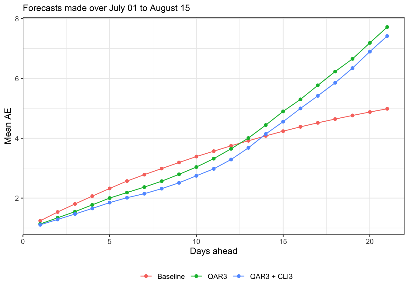
Try it out, mean AE and mean WIS
subtitle = sprintf("Forecasts made over %s to %s",
                   format(min(forecast_dates), "%B %d"),
                   format(max(forecast_dates), "%B %d"))

canonical_plot(evals, x = "ahead", y = "ae", aggr = mean,
               subtitle = subtitle, xlab = "Days ahead", ylab = "Mean AE")
canonical_plot(evals, x = "ahead", y = "wis", aggr = mean,
               subtitle = subtitle, xlab = "Days ahead", ylab = "Mean WIS")
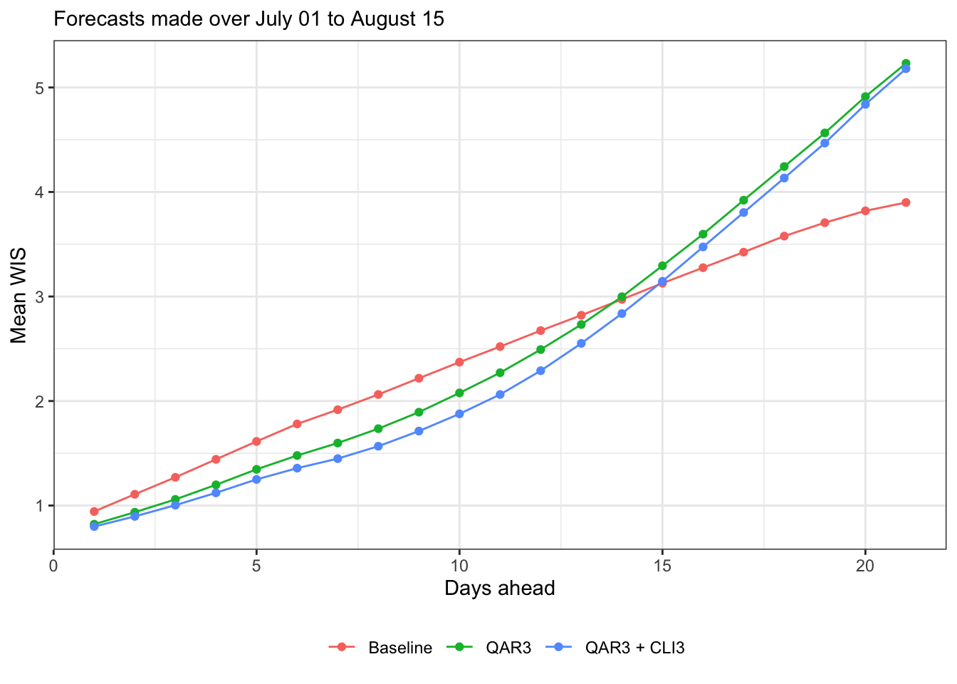
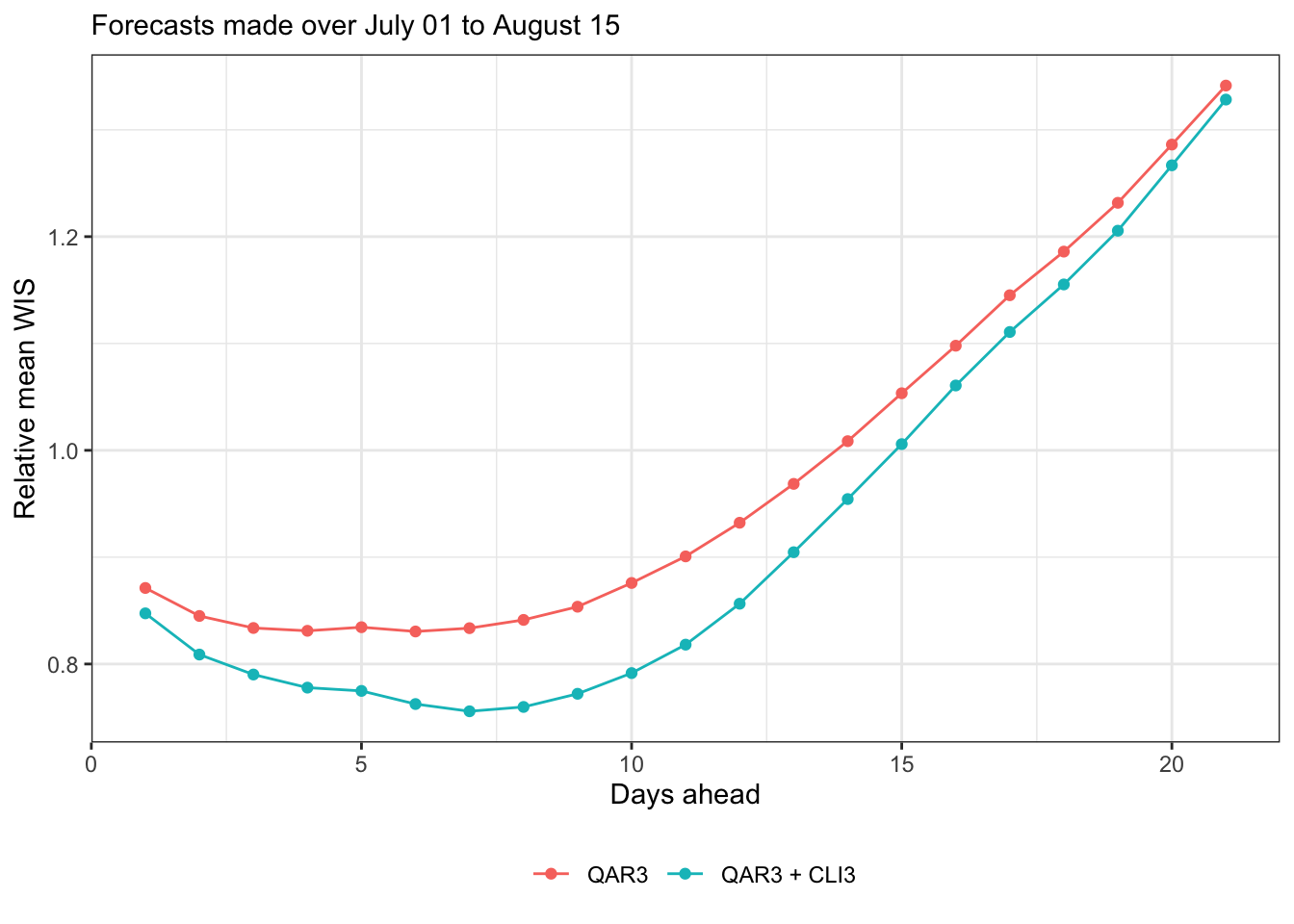
Let’s just focus on WIS from here on, since AE behaves qualitatively similarly. Here’s relative mean WIS (relative to baseline)
canonical_plot(evals, x = "ahead", y = "wis", aggr = mean,
               denom_forecaster = "Baseline", subtitle = subtitle,
               xlab = "Days ahead", ylab = "Relative mean WIS")
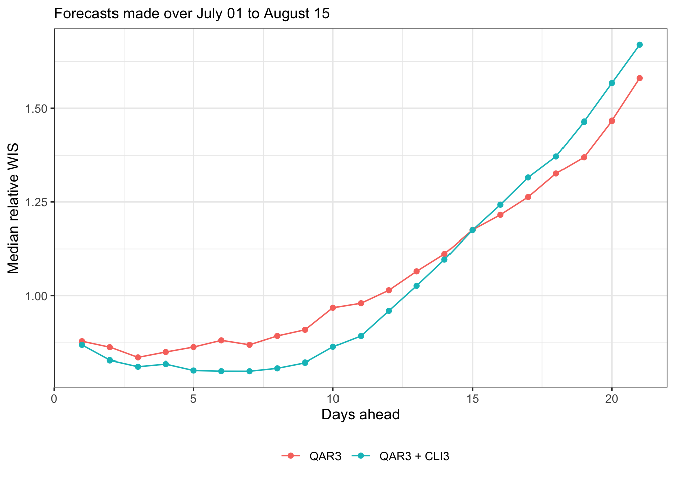
Median relative WIS (still relative to baseline; note the reversal in the order of operaitons, and median for robustness)
canonical_plot(evals, x = "ahead", y = "wis", aggr = median,
               denom = "Baseline", scale_before = TRUE, sub = subtitle,
               xlab = "Days ahead", ylab = "Median relative WIS")
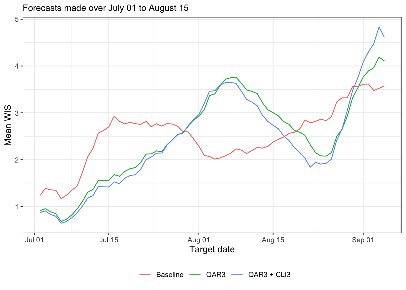
Now produce some plots of forecast scores time, i.e., by target end date
canonical_plot(evals, x = "target_end_date", y = "wis", aggr = mean,
               dots = FALSE, group_vars = "forecaster", sub = subtitle,
               xlab = "Target date", ylab = "Mean WIS")
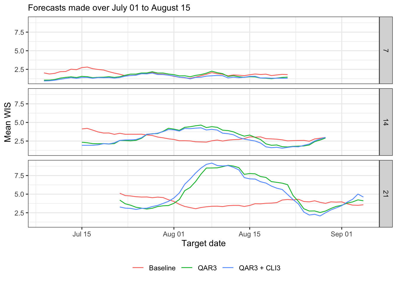
canonical_plot(evals %>% filter(ahead %in% (1:3 * 7)),
               x = "target_end_date", y = "wis", aggr = mean,
               dots = FALSE, group_vars = c("forecaster", "ahead"),
               facet_rows = "ahead", sub = subtitle,
               xlab = "Target date", ylab = "Mean WIS")
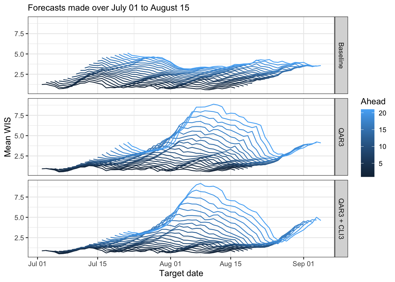
canonical_plot(evals, x = "target_end_date", y = "wis", aggr = mean,
               dots = FALSE, group_vars = c("forecaster", "ahead"),
               facet_rows = "forecaster", sub = subtitle,
               xlab = "Target date", ylab = "Mean WIS",
               legend_pos = "right", legend_title = "Ahead")
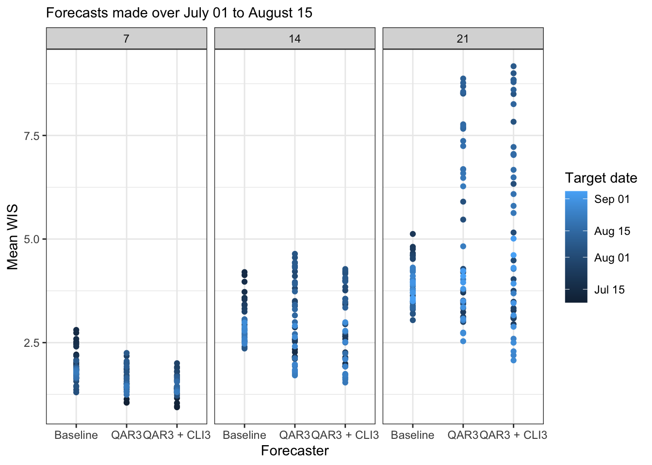
Now of a plot forecast scores broken down by target end date and ahead
canonical_plot(evals %>% filter(ahead %in% (1:3 * 7)),
               x = "forecaster", y = "wis", aggr = mean, lines = FALSE,
               group_vars = c("target_end_date", "ahead"), facet_cols = "ahead",
               sub = subtitle, xlab = "Forecaster", ylab = "Mean WIS",
               legend_position = "right", legend_title = "Target date")