Get started with epidatr • epidatr

The epidatr package provides access to all the endpoints of the Delphi Epidata API, and can be used to make requests for specific signals on specific dates and in select geographic regions. It is widely used in epidemiological research, real-time forecasting models, and public health dashboards.

Setup

Installation

You can install the stable version of this package from CRAN:

# Install from CRAN
install.packages("epidatr")
# or using pak
pak::pkg_install("epidatr")
# or using renv
renv::install("epidatr")

Or if you want the development version, install from GitHub:

# Install the dev version using pak
pak::pkg_install("cmu-delphi/epidatr@dev")
# or using remotes
remotes::install_github("cmu-delphi/epidatr", ref = "dev")
# or using renv
renv::install("cmu-delphi/epidatr@dev")

API Keys

The Delphi API requires a (free) API key for full functionality. While most endpoints are available without one, there are limits on API usage for anonymous users, including a rate limit.

To generate your key, register for a pseudo-anonymous account. See the save_api_key() function documentation for details on how to set up epidatr to use your API key.

The Delphi V5 API

Epidatr allows three categories of data access to the Delphi V5 API:

epidata_snapshot() provides a specific view of how a dataset looked at a point in time.
epidata_archive() fetches all versions of a dataset across time, representing the full revision history.
epidata_aux() accesses source-specific auxiliary tables containing metadata, laboratory protocols, or additional static keys (such as NWSS wastewater facility descriptions).

Additionally, epidata_meta() provides access to system metadata to list available sources, signals, geographic granularities, and date ranges.

Basic Usage

To make a request of a particular data source at a specific point in time, we’ll use epidata_snapshot(). This function needs the source name, signal name, and a geographic level in order to complete a query.

Suppose we are interested in the nssp source, which provides access to a wide range of emergency department visits data:

library(epidatr)
library(dplyr)
#> Warning: package 'dplyr' was built under R version 4.5.2
#> 
#> Attaching package: 'dplyr'
#> The following objects are masked from 'package:stats':
#> 
#>     filter, lag
#> The following objects are masked from 'package:base':
#> 
#>     intersect, setdiff, setequal, union

# Obtain the latest snapshot of the influenza ED-visit percentage
# from the NSSP source for the US
epidata <- epidata_snapshot(
  source = "nssp",
  signals = "pct_ed_visits_influenza",
  geo_type = "nation"
)
knitr::kable(head(epidata))

signal	report_time	geo_type	geo_value	fill_method	reference_time	value
pct_ed_visits_influenza	2026-06-26	nation	us	source	2022-10-01	0.48
pct_ed_visits_influenza	2026-06-26	nation	us	source	2022-10-08	0.67
pct_ed_visits_influenza	2026-06-26	nation	us	source	2022-10-15	0.90
pct_ed_visits_influenza	2026-06-26	nation	us	source	2022-10-22	1.29
pct_ed_visits_influenza	2026-06-26	nation	us	source	2022-10-29	2.47
pct_ed_visits_influenza	2026-06-26	nation	us	source	2022-11-05	3.67

epidata_snapshot() returns a tibble (a modern reimagining of R’s standard data frame that prints cleanly and preserves typed columns). (Here we’re using knitr::kable() to make it more readable.) Each row represents one observation for the US on one date. The location is given in the geo_value column, the date it describes in the reference_time column, the value of the requested signal in value, and the publication date in report_time.

The Delphi V5 API makes signals available at different geographic levels, depending on the source. Use epidata_meta("nssp") for a given source to see which geo types it supports.

To request signals for all states instead of the entire US, we use the geo_type argument. This automatically returns all available data for that geo type:

# Obtain the latest snapshot of the influenza ED-visit percentage
# from the NSSP source across all available dates and states
epidata_snapshot(
  source = "nssp",
  signals = "pct_ed_visits_influenza",
  geo_type = "state"
)
#> # A tibble: 10,557 × 7
#>   signal         report_time geo_type geo_value fill_method reference_time value
#>   <chr>          <date>      <chr>    <chr>     <chr>       <date>         <dbl>
#> 1 pct_ed_visits… 2026-06-26  state    ak        source      2022-10-01     0.140
#> 2 pct_ed_visits… 2026-06-26  state    ak        source      2022-10-08     0.240
#> 3 pct_ed_visits… 2026-06-26  state    ak        source      2022-10-15     0.320
#> 4 pct_ed_visits… 2026-06-26  state    ak        source      2022-10-22     0.760
#> # ℹ 10,553 more rows

You can also query multiple signals in a single request by passing a vector to signals:

# Obtain both influenza and COVID-19 ED-visit percentages in a single query
epidata_snapshot(
  source = "nssp",
  signals = c("pct_ed_visits_influenza", "pct_ed_visits_covid"),
  geo_type = "state",
  geo_values = "pa",
  reference_time = epirange("2024-12-01", "2024-12-15")
)
#> # A tibble: 4 × 7
#>   signal         report_time geo_type geo_value fill_method reference_time value
#>   <chr>          <date>      <chr>    <chr>     <chr>       <date>         <dbl>
#> 1 pct_ed_visits… 2026-06-26  state    pa        source      2024-12-07     0.75 
#> 2 pct_ed_visits… 2026-06-26  state    pa        source      2024-12-07     0.570
#> 3 pct_ed_visits… 2026-06-26  state    pa        source      2024-12-14     0.820
#> 4 pct_ed_visits… 2026-06-26  state    pa        source      2024-12-14     0.870

Alternatively, we can fetch the time series for a subset of states and reference dates by listing out the desired locations in the geo_values argument and using a range in the reference_time argument:

# Obtain the data from January 1st, 2024 to January 1st, 2025
# of the influenza ED-visit percentage from the NSSP source for 
# Pennsylvania, California, and Florida
epidata_snapshot(
  source = "nssp",
  signals = "pct_ed_visits_influenza",
  geo_type = "state",
  geo_values = c("pa", "ca", "fl"),
  reference_time = epirange("2024-01-01", "2025-01-01")
)
#> # A tibble: 156 × 7
#>   signal         report_time geo_type geo_value fill_method reference_time value
#>   <chr>          <date>      <chr>    <chr>     <chr>       <date>         <dbl>
#> 1 pct_ed_visits… 2026-06-26  state    ca        source      2024-02-03     1.31 
#> 2 pct_ed_visits… 2026-06-26  state    ca        source      2024-02-17     0.990
#> 3 pct_ed_visits… 2026-06-26  state    ca        source      2024-03-02     0.760
#> 4 pct_ed_visits… 2026-06-26  state    ca        source      2024-03-09     0.650
#> # ℹ 152 more rows

Getting versioned data

The Delphi V5 API stores a historical record of all data, including corrections and updates, which is particularly useful for accurately backtesting forecasting models. To retrieve versioned data in epidata_snapshot(), we can use the snapshot_date argument, which fetches the data as it was known on a specific date.

# Obtain the influenza ED-visit percentage from NSSP for Pennsylvania
# as it was known on 2025-01-01
epidata_snapshot(
  source = "nssp",
  signals = "pct_ed_visits_influenza",
  geo_type = "state",
  geo_values = "pa",
  snapshot_date = "2025-01-01"
)
#> # A tibble: 117 × 7
#>   signal         report_time geo_type geo_value fill_method reference_time value
#>   <chr>          <date>      <chr>    <chr>     <chr>       <date>         <dbl>
#> 1 pct_ed_visits… 2024-12-27  state    pa        source      2022-10-01     0.120
#> 2 pct_ed_visits… 2024-12-27  state    pa        source      2022-10-08     0.100
#> 3 pct_ed_visits… 2024-12-27  state    pa        source      2022-10-15     0.210
#> 4 pct_ed_visits… 2024-12-27  state    pa        source      2022-10-22     0.330
#> # ℹ 113 more rows

To request all versions of the data issued within a specific time range, we use epidata_archive() with the report_time argument. This parameter allows us to fetch versions using comparison operators (e.g., "<2025-01-15>") or an epirange().

# See how the estimate for a SINGLE reference date (2024-12-07) evolved
# by fetching all reports issued in December 2024 and early January 2025
epidata_archive(
  source = "nssp",
  signals = "pct_ed_visits_influenza",
  geo_type = "state",
  geo_values = "pa",
  reference_time = "2024-12-07",
  report_time = epirange("2024-12-01", "2025-01-15")
)
#> # A tibble: 5 × 7
#>   signal         report_time geo_type geo_value fill_method reference_time value
#>   <chr>          <date>      <chr>    <chr>     <chr>       <date>         <dbl>
#> 1 pct_ed_visits… 2024-12-13  state    pa        source      2024-12-07     0.550
#> 2 pct_ed_visits… 2024-12-20  state    pa        source      2024-12-07     0.560
#> 3 pct_ed_visits… 2024-12-27  state    pa        source      2024-12-07     0.560
#> 4 pct_ed_visits… 2025-01-03  state    pa        source      2024-12-07     0.560
#> # ℹ 1 more row

See vignette("versioned-data") for details and more ways to specify versioned data.

Auxiliary data

Some sources include extra columns connected to the signal data, such as the population served by each NWSS sewershed or site metadata. epidata_aux() retrieves this auxiliary data, either on its own or merged onto a signal pull.

You can pull auxiliary data directly by source. To see what key columns you can filter on for a given source, consult that source’s page in the V5 signals documentation. Named filters on these key columns can be passed through ... to limit the returned rows, and columns can be used to select specific fields:

aux_data <- epidata_aux(
  source = "nwss",
  pcr_target = "sars-cov-2",
  sample_index = c("92012", "92013")
)
knitr::kable(head(aux_data))

report_time	geo_value	reference_time	nwss_source	sample_index	pcr_target	report_ts_nominal_end	state_territory	county_fips	counties_served	population_served	sample_type	sample_matrix	sample_location	flow_rate	concentration_method	pasteurized	pcr_type	extraction_method	major_lab_method	inhibition_detect	inhibition_adjust	ntc_amplify	pcr_gene_target_agg	pcr_target_units	lod_sewage	hum_frac_target_mic	hum_frac_mic_conc	hum_frac_mic_unit	rec_eff_percent	rec_eff_target_name	rec_eff_spike_matrix	rec_eff_spike_conc	pipeline_run_id	report_ts_actual	comments
2026-06-26	162	2026-01-27	CDC_Verily	92012	sars-cov-2	NA	ca	06079	San Luis Obispo	14465	24-hr time-weighted composite	post grit removal	wwtp	0.45	ceres nanotrap	f	ddpcr	thermo magmax viral/pathogen nucleic acid isolation kit	2	f	f	f	n	copies/l wastewater	1500	pepper mild mottle virus	153424325.78462	copies/l wastewater	40.7	bcov vaccine	clarified sample	5	7914	2026-06-26 21:04:11	NA
2026-06-19	162	2026-01-27	CDC_Verily	92012	sars-cov-2	2026-06-26 00:00:00	ca	06079	San Luis Obispo	14465	24-hr time-weighted composite	post grit removal	wwtp	0.45	ceres nanotrap	f	ddpcr	thermo magmax viral/pathogen nucleic acid isolation kit	2	f	f	f	n	copies/l wastewater	1500	pepper mild mottle virus	153424325.78462	copies/l wastewater	40.7	bcov vaccine	clarified sample	5	7895	2026-06-26 21:02:14	NA
2026-06-12	162	2026-01-27	CDC_Verily	92012	sars-cov-2	2026-06-19 00:00:00	ca	06079	San Luis Obispo	14465	24-hr time-weighted composite	post grit removal	wwtp	0.45	ceres nanotrap	f	ddpcr	thermo magmax viral/pathogen nucleic acid isolation kit	2	f	f	f	n	copies/l wastewater	1500	pepper mild mottle virus	153424325.78462	copies/l wastewater	40.7	bcov vaccine	clarified sample	5	7879	2026-06-26 21:00:39	NA
2026-06-05	162	2026-01-27	CDC_Verily	92012	sars-cov-2	2026-06-12 00:00:00	ca	06079	San Luis Obispo	14465	24-hr time-weighted composite	post grit removal	wwtp	0.45	ceres nanotrap	f	ddpcr	thermo magmax viral/pathogen nucleic acid isolation kit	2	f	f	f	n	copies/l wastewater	1500	pepper mild mottle virus	153424325.78462	copies/l wastewater	40.7	bcov vaccine	clarified sample	5	7868	2026-06-26 20:59:33	NA
2026-05-30	162	2026-01-27	CDC_Verily	92012	sars-cov-2	2026-06-05 00:00:00	ca	06079	San Luis Obispo	14465	24-hr time-weighted composite	post grit removal	wwtp	0.45	ceres nanotrap	f	ddpcr	thermo magmax viral/pathogen nucleic acid isolation kit	2	f	f	f	n	copies/l wastewater	1500	pepper mild mottle virus	153424325.78462	copies/l wastewater	40.7	bcov vaccine	clarified sample	5	7858	2026-06-26 20:58:46	NA
2026-05-29	162	2026-01-27	CDC_Verily	92012	sars-cov-2	2026-05-30 00:00:00	ca	06079	San Luis Obispo	14465	24-hr time-weighted composite	post grit removal	wwtp	0.45	ceres nanotrap	f	ddpcr	thermo magmax viral/pathogen nucleic acid isolation kit	2	f	f	f	n	copies/l wastewater	1500	pepper mild mottle virus	153424325.78462	copies/l wastewater	40.7	bcov vaccine	clarified sample	5	7847	2026-06-26 20:57:31	NA

You can also attach auxiliary columns directly to a signal pull by passing the output of epidata_snapshot() or epidata_archive() directly to epidata_aux(). In this workflow, epidata_aux() fetches the matching auxiliary data and left-joins it onto the shared key columns:

# Fetch signal data for a specific sewershed
nwss_data <- epidata_snapshot(
  source = "nwss",
  signals = "covid_avg_conc",
  geo_type = "sewershed",
  geo_values = "128",
  reference_time = epirange("2024-12-01", "2025-01-01")
)
head(nwss_data)
#> # A tibble: 6 × 10
#>   signal   report_time geo_type geo_value fill_method reference_time nwss_source
#>   <chr>    <date>      <chr>    <chr>     <chr>       <date>         <chr>      
#> 1 covid_a… 2026-06-26  sewersh… 128       source      2024-12-19     CDC_Verily 
#> 2 covid_a… 2026-06-26  sewersh… 128       source      2024-12-03     CDC_Verily 
#> 3 covid_a… 2026-06-26  sewersh… 128       source      2024-12-17     CDC_Verily 
#> 4 covid_a… 2026-06-26  sewersh… 128       source      2024-12-12     CDC_Verily 
#> # ℹ 2 more rows
#> # ℹ 3 more variables: sample_index <chr>, pcr_target <chr>, value <dbl>

# Attach auxiliary metadata
nwss_merged <- nwss_data %>%
  epidata_aux()
head(nwss_merged)
#> # A tibble: 6 × 40
#>   signal   report_time geo_type geo_value fill_method reference_time nwss_source
#>   <chr>    <date>      <chr>    <chr>     <chr>       <date>         <chr>      
#> 1 covid_a… 2026-06-26  sewersh… 128       source      2024-12-19     CDC_Verily 
#> 2 covid_a… 2026-06-26  sewersh… 128       source      2024-12-03     CDC_Verily 
#> 3 covid_a… 2026-06-26  sewersh… 128       source      2024-12-17     CDC_Verily 
#> 4 covid_a… 2026-06-26  sewersh… 128       source      2024-12-12     CDC_Verily 
#> # ℹ 2 more rows
#> # ℹ 33 more variables: sample_index <chr>, pcr_target <chr>, value <dbl>,
#> #   report_ts_nominal_end <chr>, state_territory <chr>, county_fips <chr>,
#> #   counties_served <chr>, population_served <chr>, sample_type <chr>,
#> #   sample_matrix <chr>, sample_location <chr>, flow_rate <chr>,
#> #   concentration_method <chr>, pasteurized <chr>, pcr_type <chr>,
#> #   extraction_method <chr>, major_lab_method <chr>, inhibition_detect <chr>, …

If you don’t pass explicit key filters, epidata_aux() automatically infers them from the base dataset.

Advanced queries

Server-side key filtering

Beyond standard arguments (source, signals, geo_type), some sources include extra key dimensions that categorize the data (for example, nwss categorizes by pcr_target, and pophive categorizes by age_group). To see what key columns are available per source, consult that source’s page in the V5 signals documentation. You can pass these extra dimensions directly as named parameters to filter the query server-side:

epidata_snapshot(
  source = "nwss",
  signals = "pcr_conc_smoothed",
  geo_type = "county",
  pcr_target = c("sars-cov-2", "influenza")
)

Dry runs

If you want to inspect the generated API request URL underlying each function query without actually fetching data, you can pass dry_run = TRUE via fetch_args_list(). This works with epidata_snapshot(), epidata_archive(), and epidata_aux():

dry_run_call <- epidata_snapshot(
  source = "nssp",
  signals = "pct_ed_visits_influenza",
  geo_type = "state",
  fetch_args = fetch_args_list(dry_run = TRUE)
)
dry_run_call
#> 
#> ── <epidata_call> object: ──────────────────────────────────────────────────────
#> • Pipe this object into `fetch()` to actually fetch the data
#> • Request URL:
#>   https://delphi.cmu.edu/epidata/v5/snapshot/?source=nssp&signal=pct_ed_visits_influenza&geo_type=state

Plotting

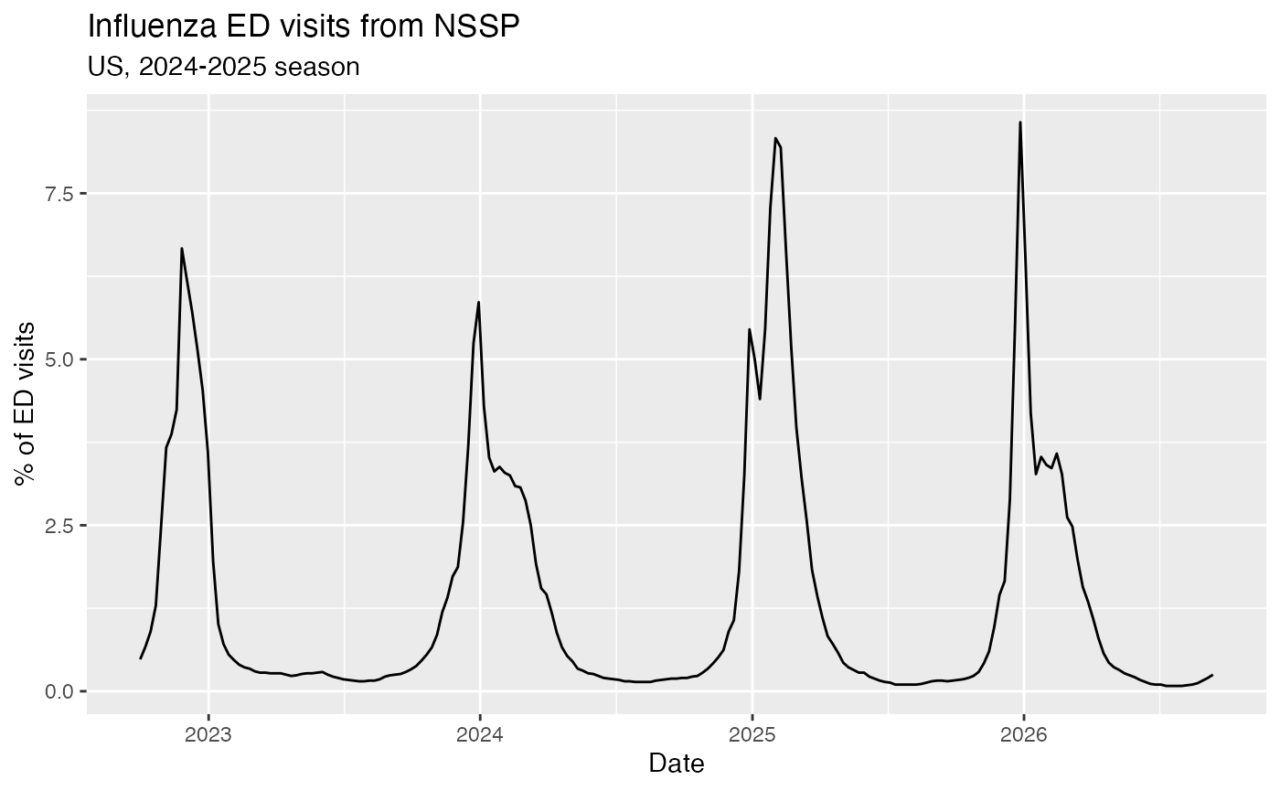
Because the output data is in a standard tibble format, we can easily plot it using ggplot2:

library(ggplot2)
#> Warning: package 'ggplot2' was built under R version 4.5.2

# Plot the influenza ED-visit time series fetched earlier with epidata_snapshot()
ggplot(epidata, aes(x = reference_time, y = value)) +
  geom_line() +
  labs(
    title = "Influenza ED visits from NSSP",
    subtitle = "US, 2024-2025 season",
    x = "Date",
    y = "% of ED visits"
  )

plot of chunk unnamed-chunk-12

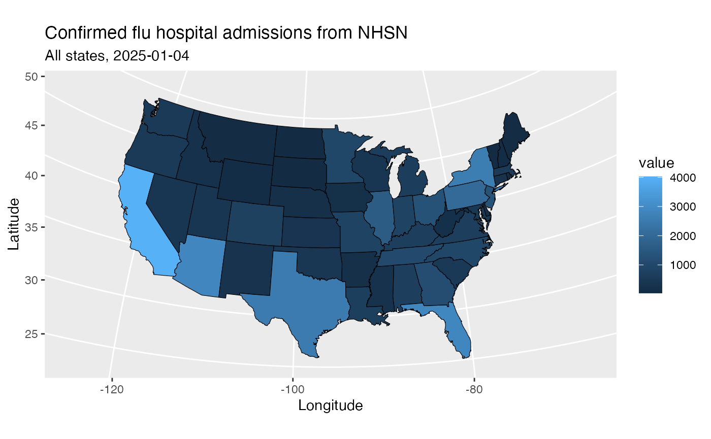
ggplot2 can also be used with epidatr and maps to create choropleths:

library(epidatr)
library(dplyr)
library(ggplot2)
library(maps)

# Obtain the latest snapshot of confirmed flu hospital admissions
# from NHSN for all states on a single reference date
nhsn_states <- epidata_snapshot(
  source = "nhsn",
  signals = "confirmed_admissions_flu_ew",
  geo_type = "state",
  geo_values = "*",
  reference_time = "2025-01-04"
)

# Get a mapping of states to longitude/latitude coordinates
states_map <- map_data("state")

# Convert state abbreviations into state names
nhsn_states <- mutate(
  nhsn_states,
  state = ifelse(
    geo_value == "dc",
    "district of columbia",
    state.name[match(geo_value, tolower(state.abb))] %>% tolower()
  )
)

# Add coordinates for each state
nhsn_states <- left_join(states_map, nhsn_states, by = c("region" = "state"))

# Plot
ggplot(nhsn_states, aes(x = long, y = lat, group = group, fill = value)) +
  geom_polygon(colour = "black", linewidth = 0.2) +
  coord_map("polyconic") +
  labs(
    title = "Confirmed flu hospital admissions from NHSN",
    subtitle = "All states, 2025-01-04",
    x = "Longitude",
    y = "Latitude"
  )

plot of chunk unnamed-chunk-13

Plotting revision histories

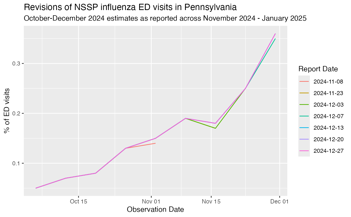
We can also visualize revision histories from epidata_archive(). Each line shows what the time series looked like as of a different publication date:

# Fetch revision history for Pennsylvania influenza ED visits
pa_revisions <- epidata_archive(
  source = "nssp",
  signals = "pct_ed_visits_influenza",
  geo_type = "state",
  geo_values = "pa",
  reference_time = epirange("2024-10-01", "2024-12-01"),
  report_time = epirange("2024-11-01", "2025-01-01")
)

ggplot(pa_revisions, aes(x = reference_time, y = value, group = report_time, color = as.factor(report_time))) +
  geom_line() +
  labs(
    title = "Revisions of NSSP influenza ED visits in Pennsylvania",
    subtitle = "October-December 2024 estimates as reported across November 2024 - January 2025",
    x = "Observation Date",
    y = "% of ED visits",
    color = "Report Date"
  )

plot of chunk archive-plot

Available data sources and endpoints

epidatr provides access to a broad ecosystem of epidemiological data streams:

V5 sources provide access to active surveillance data queried via epidata_snapshot() and epidata_archive(). Discover them programmatically using epidata_meta() or interactively on the Delphi EpiPortal.
Migrating endpoints are legacy endpoints (such as pub_covidcast(), pub_fluview(), pub_flusurv(), and pub_meta()) transitioning to V5. See vignette("migration-guide") for argument mappings and migration details.
Historical endpoints provide access to datasets whose collection has ended (such as Google Flu Trends, Wikipedia article views, and historical hospitalization series) kept for retrospective analysis via pub_* functions.
- International endpoints are a subset of historical datasets that focus on surveillance outside the United States (e.g., PAHO dengue with pub_paho_dengue() and ECDC ILI with pub_ecdc_ili()).
- Private endpoints are restricted streams (e.g., CDC web metrics with pvt_cdc() and digital sensors with pvt_sensors()) that require dedicated secret authentication keys.

See vignette("signal-discovery") for an in-depth guide to discovering signals, browsing metadata, and querying datasets across all these categories.