4. Combine external data sources and COVIDcast data • covidcast

While the COVIDcast Epidata API provides numerous useful COVID data streams, you may sometimes find yourself with relevant data from a different source. This package provides the tools you need to load such data and use it alongside COVIDcast data—for example, you can calculate correlations with covidcast_cor() and make maps using plot.covidcast_signal().

Let’s illustrate this in action using data from the COVID Tracking Project. They provide CSV files for download containing daily state-level data on numerous metrics, including cases, deaths, hospitalizations, and test results.

Loading the data

We’ve saved a sample of the data in this package to use as an example. Let’s load it and examine a few columns using knitr::kable() to print them nicely:

library(dplyr)

data <- read.csv(system.file("extdata", "covid-tracking-project-oct-2020.csv",
                             package = "covidcast", mustWork = TRUE))

data %>%
    select(date, state, death, deathIncrease, hospitalizedCurrently,
           hospitalizedIncrease) %>%
    head() %>%
    knitr::kable()

date	state	death	deathIncrease	hospitalizedCurrently	hospitalizedIncrease
2020-10-31	AK	82	1	94	7
2020-10-31	AL	2967	35	960	0
2020-10-31	AR	1925	25	652	35
2020-10-31	AS	0	0	NA	0
2020-10-31	AZ	5979	45	889	68
2020-10-31	CA	17626	55	3212	0

This is in a convenient format: Each day’s observations for each state are in one row. Suppose we would like to extract hospitalizedIncrease as a signal we want to map and analyze alongside other data fetched with covidcast_signal().

To do this, we use as.covidcast_signal(). It expects a data frame with at least three columns:

time_value: a Date object giving the observation date
value: the value of the observation, such as the number of deaths or hospitalizations
geo_value: the location, such as state or county, in the same form as returned by covidcast_signal() (such as two-letter lowercase abbreviations for states and FIPS codes for counties)

Other columns are preserved unchanged. (In particular, if an issue column is present, it is used as the issue date of each observation. This is important if your data source includes multiple revisions of each observation.) as.covidcast_signal() also needs to know the geo_type (state, in this case) and source/signal name to apply to the data. With a bit of dplyr data wrangling, we can do this easily:

library(covidcast)

hospitalized <- data %>%
    select(time_value = date,
           geo_value = state,
           value = hospitalizedIncrease) %>%
    mutate(geo_value = tolower(geo_value),
           time_value = as.Date(time_value)) %>%
    as.covidcast_signal(geo_type = "state",
                        data_source = "covid-tracking",
                        signal = "hospitalized_increase")

head(hospitalized) %>%
    knitr::kable()

data_source	signal	geo_value	time_value	value	issue
covid-tracking	hospitalized_increase	ak	2020-10-31	7	2023-07-12
covid-tracking	hospitalized_increase	al	2020-10-31	0	2023-07-12
covid-tracking	hospitalized_increase	ar	2020-10-31	35	2023-07-12
covid-tracking	hospitalized_increase	as	2020-10-31	0	2023-07-12
covid-tracking	hospitalized_increase	az	2020-10-31	68	2023-07-12
covid-tracking	hospitalized_increase	ca	2020-10-31	0	2023-07-12

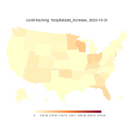
This allows us to make maps using the same functions used for other COVIDcast data:

plot(hospitalized, plot_type = "choro")

Warning: Metadata for signal mean and standard deviation not available;
defaulting to observed mean and standard deviation to set plot range.

Analysis alongside other signals

Now that our data is loaded as a covidcast_signal object, we can use it alongside other signals from the API. For example, let’s examine how new COVID hospitalizations correlate with outpatient doctor visits with deaths during October 2020, where we use death data as reported by the API.

deaths <- covidcast_signal("jhu-csse", "deaths_7dav_incidence_prop",
                           start_day = "2020-10-01",
                           end_day = "2020-10-31",
                           geo_type = "state")

covidcast_cor(deaths, hospitalized, by = "time_value")

# A tibble: 31 × 2
   time_value  value
   <date>      <dbl>
 1 2020-10-01 0.218 
 2 2020-10-02 0.120 
 3 2020-10-03 0.147 
 4 2020-10-04 0.148 
 5 2020-10-05 0.0436
 6 2020-10-06 0.0706
 7 2020-10-07 0.123 
 8 2020-10-08 0.0300
 9 2020-10-09 0.0955
10 2020-10-10 0.178 
# ℹ 21 more rows

We can also use the tools provided by this package to place both signals into a single data frame for analysis. For example, to build a model that uses hospitalizations and other data to predict deaths, it may be convenient to produce a data frame where each row represents one state on one day, and each column is a variable (such as hospitalization or death). Using aggregate_signals(), this is easy:

death_hosp <- aggregate_signals(list(deaths, hospitalized),
                                format = "wide")

head(death_hosp) %>%
    knitr::kable()

geo_value	time_value	value+0:jhu-csse_deaths_7dav_incidence_prop
ca	2020-10-01	0.2286116
ca	2020-10-02	0.2137337
ca	2020-10-03	0.2122822
ca	2020-10-04	0.2122822
ca	2020-10-05	0.2177254
ca	2020-10-06	0.1788977