The evalcast package provides the infrastructure for developing and evaluating probabilistic forecasters that are based on data obtained with the covidcast R package. A unique feature of the covidcast API is that it can retrieve data that would have been available as of a certain date. This accounts for a difficult property of working with certain COVID-19 data sources, which is that they may be backfilled (retrospectively updated). Failing to account for backfill can lead to poorly trained forecasters and overly optimistic retrospective evaluations. The evalcast package is designed to help forecasters avoid these pitfalls.
Testing forecasters
We will use the included baseline_forecaster to demonstrate how to backtest a forecaster and compare its predictions to contemporaneous forecasts that were submitted to CovidHub. While baseline_forecaster is very simple, it can be used as a template for creating more sophisticated forecasters.
The format of a forecaster is aligned with the CovidHub submission instructions and with the covidcast R package.
Specify the signals that will be used by forecaster
We start by specifying which signals the forecaster will be using. See here for a full list of signals available through the covidcast API. Each signal is specified by two strings: data_source and signal. Optionally, we can specify how far back in time we will want data.
library(tibble)
library(dplyr)
library(magrittr)
library(ggplot2)
signals <- tibble(data_source = "jhu-csse",
                  signal = "deaths_incidence_num",
                  start_day = "2020-06-15",
                  geo_type = "state")
signals
#> # A tibble: 1 x 4
#>   data_source signal               start_day  geo_type
#>   <chr>       <chr>                <chr>      <chr>
#> 1 jhu-csse    deaths_incidence_num 2020-06-15 state
Run the forecaster on some dates
Within the evalcast framework, forecasters do not directly retrieve historic data. Instead, get_predictions provides only the data that would have been available at the time to the specified forecaster in order to generate retrospective predictions.
library(evalcast)
library(covidcast)
library(lubridate)
library(dplyr)

forecast_dates <- get_covidhub_forecast_dates("CMU-TimeSeries")
forecast_dates_dec <- forecast_dates[forecast_dates >= "2020-12-01" &
                                        forecast_dates <= "2020-12-31"]

# Retrieve past predictions from CovidHub...
predictions_cards_ens <- get_covidhub_predictions(
  "COVIDhub-ensemble", as_date(forecast_dates_dec), ahead = 3,
  signal = "deaths_incidence_num") %>%
  filter(nchar(geo_value)==2) # remove counties
predictions_cards_cmu <- get_covidhub_predictions(
  "CMU-TimeSeries", forecast_dates_dec,  ahead = 3,
  signal = "deaths_incidence_num")
# ...or make new predictions using baseline_forecaster
predictions_cards <- get_predictions(baseline_forecaster,
                                     name_of_forecaster = "baseline",
                                     signals = signals,
                                     forecast_dates = forecast_dates_dec,
                                     incidence_period = "epiweek",
                                     forecaster_args = list(
                                       ahead = 3
                                     )
)

predictions <- bind_rows(predictions_cards, predictions_cards_cmu,
                         predictions_cards_ens)
get_predictions() and get_covidhub_predictions() return a long data frame with one row for each (forecast date, ahead, geo_value, quantile) combination.
head(predictions_cards_cmu, n=25)
#>    ahead geo_value quantile value     forecaster forecast_date data_source
#> 1      3        al    0.010   148 CMU-TimeSeries    2020-12-28    jhu-csse
#> 2      3        al    0.025   184 CMU-TimeSeries    2020-12-28    jhu-csse
#> 3      3        al    0.050   213 CMU-TimeSeries    2020-12-28    jhu-csse
#> 4      3        al    0.100   237 CMU-TimeSeries    2020-12-28    jhu-csse
#> 5      3        al    0.150   253 CMU-TimeSeries    2020-12-28    jhu-csse
#> 6      3        al    0.200   271 CMU-TimeSeries    2020-12-28    jhu-csse
#> 7      3        al    0.250   283 CMU-TimeSeries    2020-12-28    jhu-csse
#> 8      3        al    0.300   296 CMU-TimeSeries    2020-12-28    jhu-csse
#> 9      3        al    0.350   307 CMU-TimeSeries    2020-12-28    jhu-csse
#> 10     3        al    0.400   320 CMU-TimeSeries    2020-12-28    jhu-csse
#> 11     3        al    0.450   328 CMU-TimeSeries    2020-12-28    jhu-csse
#> 12     3        al    0.500   339 CMU-TimeSeries    2020-12-28    jhu-csse
#> 13     3        al    0.550   351 CMU-TimeSeries    2020-12-28    jhu-csse
#> 14     3        al    0.600   359 CMU-TimeSeries    2020-12-28    jhu-csse
#> 15     3        al    0.650   370 CMU-TimeSeries    2020-12-28    jhu-csse
#> 16     3        al    0.700   381 CMU-TimeSeries    2020-12-28    jhu-csse
#> 17     3        al    0.750   395 CMU-TimeSeries    2020-12-28    jhu-csse
#> 18     3        al    0.800   410 CMU-TimeSeries    2020-12-28    jhu-csse
#> 19     3        al    0.850   424 CMU-TimeSeries    2020-12-28    jhu-csse
#> 20     3        al    0.900   443 CMU-TimeSeries    2020-12-28    jhu-csse
#> 21     3        al    0.950   477 CMU-TimeSeries    2020-12-28    jhu-csse
#> 22     3        al    0.975   506 CMU-TimeSeries    2020-12-28    jhu-csse
#> 23     3        al    0.990   540 CMU-TimeSeries    2020-12-28    jhu-csse
#> 24     3        ak    0.010     0 CMU-TimeSeries    2020-12-28    jhu-csse
#> 25     3        ak    0.025     0 CMU-TimeSeries    2020-12-28    jhu-csse
#>                  signal target_end_date incidence_period
#> 1  deaths_incidence_num      2021-01-16          epiweek
#> 2  deaths_incidence_num      2021-01-16          epiweek
#> 3  deaths_incidence_num      2021-01-16          epiweek
#> 4  deaths_incidence_num      2021-01-16          epiweek
#> 5  deaths_incidence_num      2021-01-16          epiweek
#> 6  deaths_incidence_num      2021-01-16          epiweek
#> 7  deaths_incidence_num      2021-01-16          epiweek
#> 8  deaths_incidence_num      2021-01-16          epiweek
#> 9  deaths_incidence_num      2021-01-16          epiweek
#> 10 deaths_incidence_num      2021-01-16          epiweek
#> 11 deaths_incidence_num      2021-01-16          epiweek
#> 12 deaths_incidence_num      2021-01-16          epiweek
#> 13 deaths_incidence_num      2021-01-16          epiweek
#> 14 deaths_incidence_num      2021-01-16          epiweek
#> 15 deaths_incidence_num      2021-01-16          epiweek
#> 16 deaths_incidence_num      2021-01-16          epiweek
#> 17 deaths_incidence_num      2021-01-16          epiweek
#> 18 deaths_incidence_num      2021-01-16          epiweek
#> 19 deaths_incidence_num      2021-01-16          epiweek
#> 20 deaths_incidence_num      2021-01-16          epiweek
#> 21 deaths_incidence_num      2021-01-16          epiweek
#> 22 deaths_incidence_num      2021-01-16          epiweek
#> 23 deaths_incidence_num      2021-01-16          epiweek
#> 24 deaths_incidence_num      2021-01-16          epiweek
#> 25 deaths_incidence_num      2021-01-16          epiweek
Let’s look at one location:
michigan_abr = tolower(covidcast::name_to_abbr("Michigan")) # = "mi"
predictions_cards_cmu %>%
  filter(geo_value == michigan_abr, forecast_date == forecast_dates_dec[1]) %>%
  select(geo_value, quantile, value, forecast_date)
#>    geo_value quantile value forecast_date
#> 1         mi    0.010   370    2020-12-07
#> 2         mi    0.025   465    2020-12-07
#> 3         mi    0.050   537    2020-12-07
#> 4         mi    0.100   650    2020-12-07
#> 5         mi    0.150   721    2020-12-07
#> 6         mi    0.200   785    2020-12-07
#> 7         mi    0.250   840    2020-12-07
#> 8         mi    0.300   884    2020-12-07
#> 9         mi    0.350   919    2020-12-07
#> 10        mi    0.400   951    2020-12-07
#> 11        mi    0.450   985    2020-12-07
#> 12        mi    0.500  1022    2020-12-07
#> 13        mi    0.550  1054    2020-12-07
#> 14        mi    0.600  1085    2020-12-07
#> 15        mi    0.650  1117    2020-12-07
#> 16        mi    0.700  1159    2020-12-07
#> 17        mi    0.750  1204    2020-12-07
#> 18        mi    0.800  1248    2020-12-07
#> 19        mi    0.850  1300    2020-12-07
#> 20        mi    0.900  1363    2020-12-07
#> 21        mi    0.950  1460    2020-12-07
#> 22        mi    0.975  1545    2020-12-07
#> 23        mi    0.990  1656    2020-12-07
#> 24        mi       NA  1022    2020-12-07
Forecasts are generally probabilistic, meaning that they predict a likely distribution of values (defined by quantiles) instead of a single value. For example, on 2020-12-28 the Covidhub ensemble forecaster made the following prediction for how many cases there would be in California 3 week(s) later.
california_abr = tolower(covidcast::name_to_abbr("California")) # = "ca"
predictions_cards_ens %>%
  filter(geo_value == california_abr,
         forecast_date == forecast_dates_dec[1]) %>%
  select(quantile, value)
#>    quantile value
#> 1     0.010   742
#> 2     0.025   787
#> 3     0.050   826
#> 4     0.100   905
#> 5     0.150   935
#> 6     0.200   970
#> 7     0.250  1030
#> 8     0.300  1051
#> 9     0.350  1054
#> 10    0.400  1059
#> 11    0.450  1066
#> 12    0.500  1141
#> 13    0.550  1164
#> 14    0.600  1187
#> 15    0.650  1212
#> 16    0.700  1238
#> 17    0.750  1265
#> 18    0.800  1298
#> 19    0.850  1336
#> 20    0.900  1389
#> 21    0.950  1411
#> 22    0.975  1478
#> 23    0.990  1520
#> 24       NA  1141
An NA in the quantile column indicates a point forecast (typically the median or mean).
Evaluate the performance of a forecaster
Now that we’ve made these predictions, we’d like to know how well they perform. By default, evalcast uses the following three performance measures, but these can be easily substituted:
err_measures <- list(wis = weighted_interval_score,
                     ae = absolute_error,
                     coverage_80 = interval_coverage(coverage = 0.8))
We may now create scorecards for each forecaster’s predictions or for a filtered subset.
scorecards <- evaluate_covid_predictions(
  predictions,
  err_measures = err_measures,
  backfill_buffer = 10,
  geo_type = "state"
  )
evaluate_covid_predictions() returns a long data frame with one column for each error measure added to the predictions_cards and the quantile and value columns removed and one row for each geo_value/ahead/forecast_date/forecaster combination. If quantile predictions are needed for plotting or other downstream analysis, then use the predictions_cards.
scorecards %>% str()
#> score_cards [644 × 12] (S3: score_cards/tbl_df/tbl/data.frame)
#>  $ ahead           : int [1:644] 3 3 3 3 3 3 3 3 3 3 ...
#>  $ geo_value       : chr [1:644] "ak" "ak" "ak" "ak" ...
#>  $ forecaster      : chr [1:644] "baseline" "baseline" "baseline" "baseline" ...
#>  $ forecast_date   : Date[1:644], format: "2020-12-07" "2020-12-14" ...
#>  $ data_source     : chr [1:644] "jhu-csse" "jhu-csse" "jhu-csse" "jhu-csse" ...
#>  $ signal          : chr [1:644] "deaths_incidence_num" "deaths_incidence_num" "deaths_incidence_num" "deaths_incidence_num" ...
#>  $ target_end_date : Date[1:644], format: "2020-12-26" "2021-01-02" ...
#>  $ incidence_period: chr [1:644] "epiweek" "epiweek" "epiweek" "epiweek" ...
#>  $ actual          : num [1:644] 17 15 8 5 296 187 427 820 250 288 ...
#>  $ wis             : num [1:644] 2.351 12.203 0.978 7.633 13.185 ...
#>  $ ae              : num [1:644] 4 17 0 12 16 26 140 518 60 3 ...
#>  $ coverage_80     : num [1:644] 1 0 1 0 1 1 0 0 0 1 ...
Technical note: What does backfill_buffer = 10 do? When we evaluate a forecaster in backtesting we are assuming that we know what actually occurred. However, in light of backfill, we may not trust the data for some period of time. The argument backfill_buffer allows us to specify how many days until we believe that the data has “settled down” and is unlikely to be updated further. The choice of this argument will depend on the particular signal you are forecasting.
Plots of performance measures
evalcast provides a number of tools to visually assess a forecaster (including comparisons with other forecasters).
We can examine forecaster calibration.
plot_calibration(predictions_cards = predictions,
                 geo_type = "state", type = "wedgeplot",
                 facet_rows = "forecaster",
                 facet_cols = c("ahead", "forecast_date"))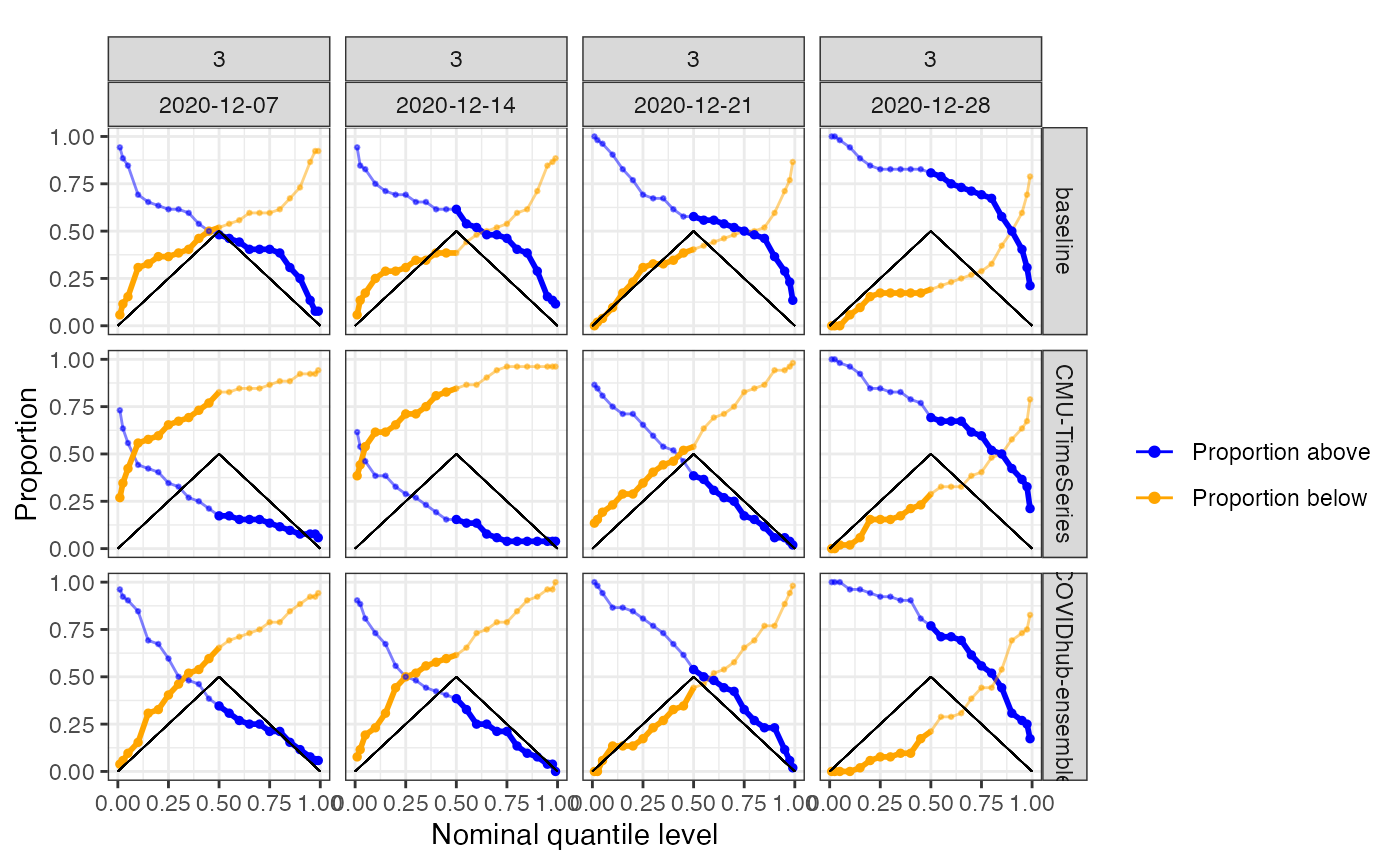
By default, the proportion is the number of geo_values that fall above/below the quantile at each forecast date and ahead, but the grouping and variables to average over can be specified.
plot_calibration(predictions_cards = predictions,
                 geo_type = "state",
                 grp_vars = "forecaster",
                 facet_cols = "forecaster",
                 avg_vars = c("geo_value", "forecast_date"),
                 facet_rows = NULL)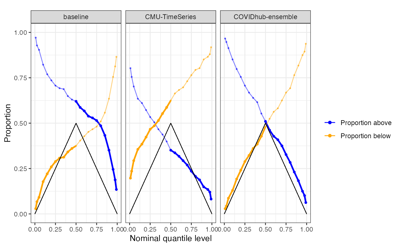
We can also examine a more traditional calibration plot:
plot_calibration(predictions_cards = predictions, geo_type = "state", type = "traditional")
For extra flexibility, you can perform the core calculations using something like:
compute_calibration(predictions, geo_type = "state") %>% setup_wedgeplot()We can display the coverage of the interval forecasts:
plot_coverage(predictions_cards = predictions,
              geo_type = "state") + theme(legend.position = "none")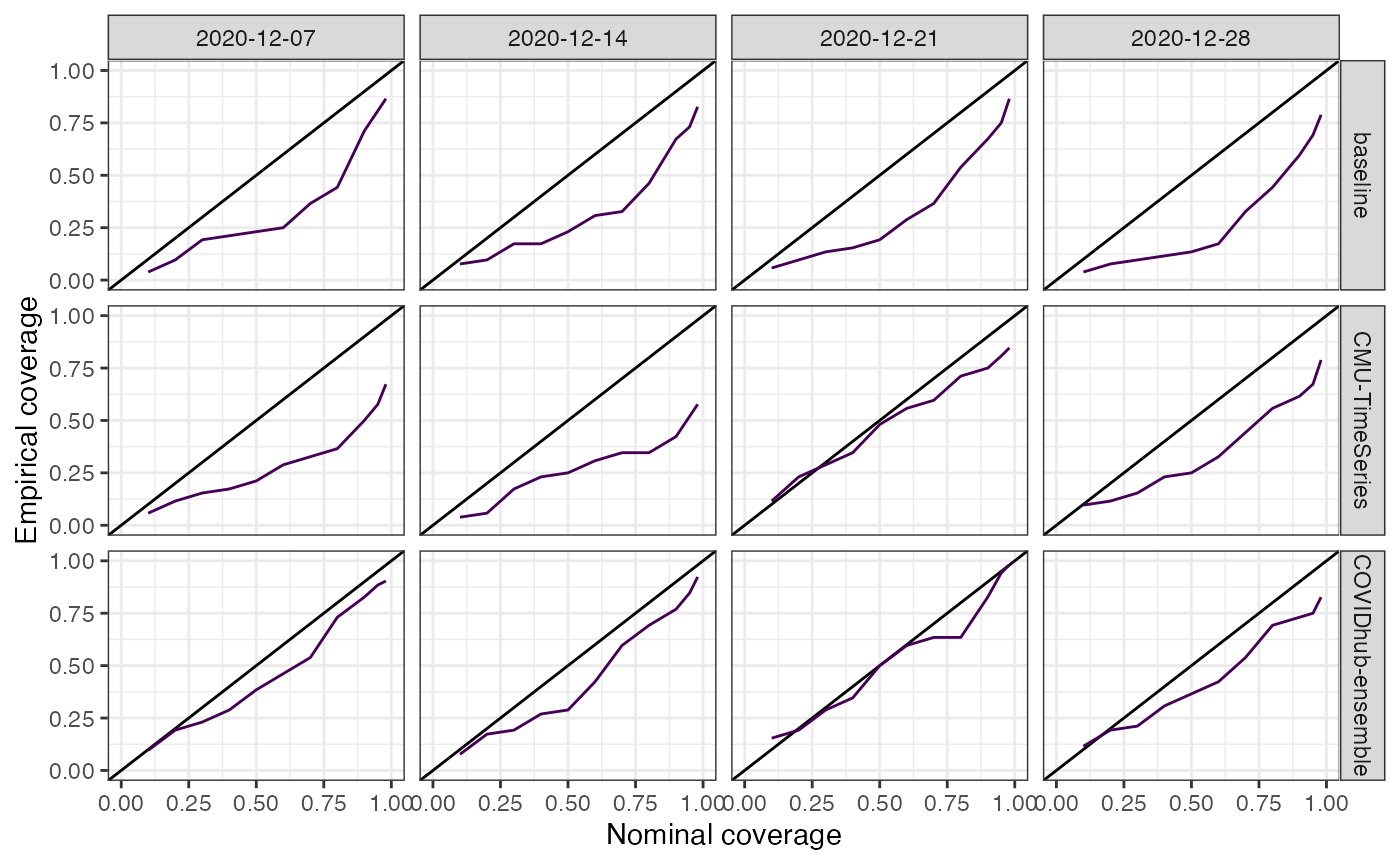
Or the width of the intervals:
plot_width(predictions_cards = predictions) + scale_y_log10() +
guides(color = "none") 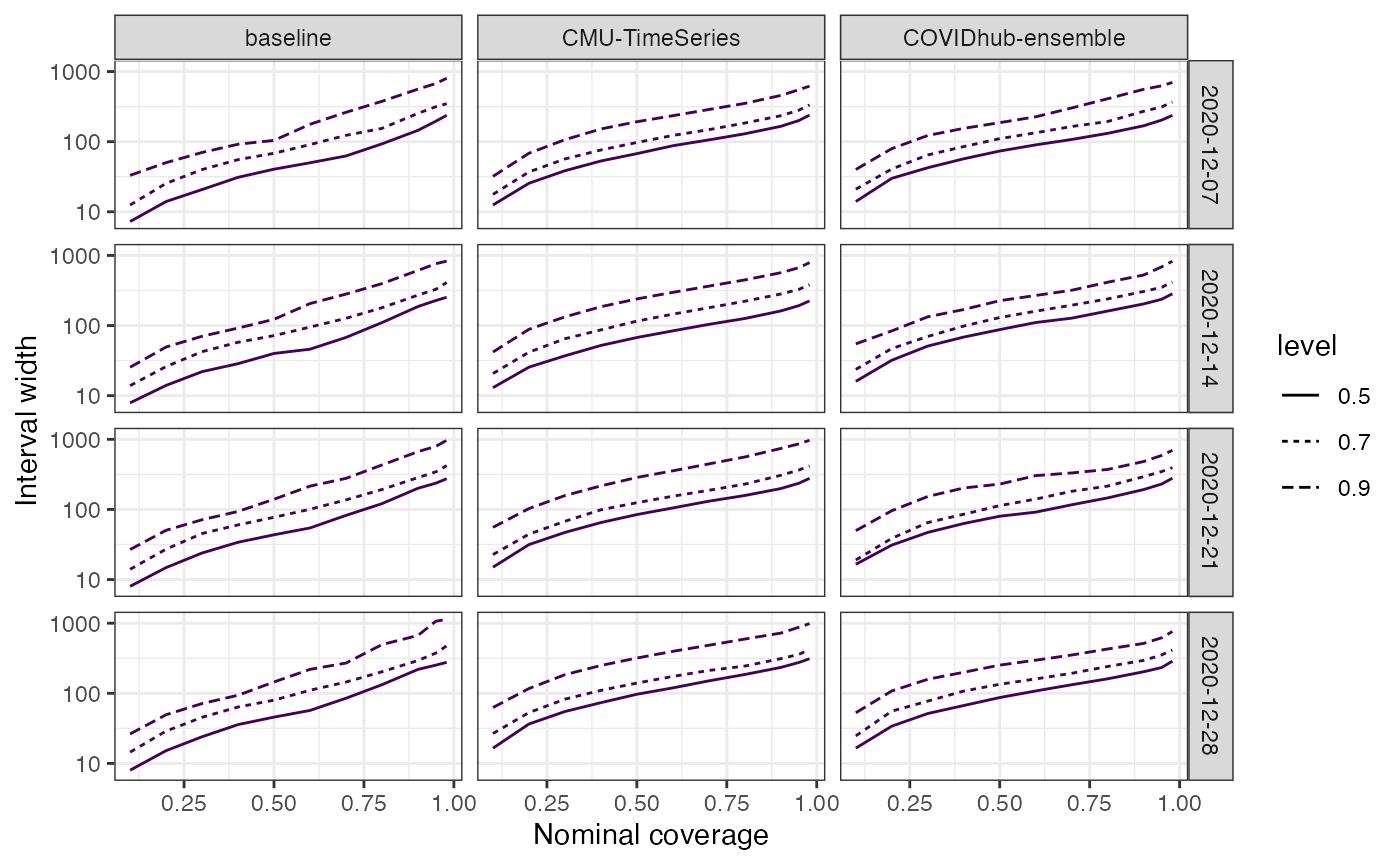
Because score_cards are just long data frames, custom plots can also be created by using {ggplot2}:
scorecards %>% filter(geo_value != "us") %>%
  ggplot(aes(y=forecaster, x=wis, fill=forecaster)) +
  geom_boxplot() +
  facet_wrap(~forecast_date) +
  scale_x_log10() +
  theme_bw() +
  scale_fill_viridis_d() +
  theme(legend.position = "bottom")
Cumulative forecasting
While the above describes incident forecasting, the same evalcast functions can also be used for cumulative forecasting.
For example, for
k-day-ahead cumulative forecasting, choose a cumulative signal fromcovidcast(e.g.,deaths_cumulative_num), setincidence_period = "day"andahead = k.For example, for
k-week-ahead cumulative epiweek forecasting, do the same as above but withahead = 7 * k.