In this vignette, we discuss how to use the sliding functionality in
the epiprocess package with less common grouping schemes or
with computations that have advanced output structures. The output of a
slide computation should either be an atomic value/vector, or a data
frame. This data frame can have multiple columns, multiple rows, or
both.
During basic usage (e.g., when all optional arguments are set to their defaults):
-
epi_slide(edf, <computation>, .....):- keeps all columns of
edf, adds computed column(s) - outputs one row per row in
edf(recycling outputs from computations appropriately if there are multiple time series bundled together inside any group(s)) - maintains the grouping or ungroupedness of
edf - is roughly analogous to (the non-sliding)
dplyr::mutatefollowed bydplyr::arrange(time_value, .by_group = TRUE) - outputs an
epi_dfif the required columns are present, otherwise a tibble
- keeps all columns of
-
epix_slide(ea, <computation>, .....):- keeps grouping and
time_valuecolumns ofea, adds computed column(s) - outputs any number of rows (computations are allowed to output any number of elements/rows, and no recycling is performed)
- maintains the grouping or ungroupedness of
ea, unless it was explicitly grouped by zero variables; this isn’t supported bygrouped_dfand it will automatically turn into an ungrouped tibble - is roughly analogous to (the non-sliding)
dplyr::group_modify - outputs a tibble
- keeps grouping and
These differences in basic behavior make some common slide operations require less boilerplate:
- predictors and targets calculated with
epi_slideare automatically lined up with each other and with the signals from which they were calculated; and - computations for an
epix_slidecan output data frames with any number of rows, containing models, forecasts, evaluations, etc., and will not be recycled.
When using more advanced features, more complex rules apply:
- Generalization:
epi_slide(edf, ....., ref_time_values=my_ref_time_values)will output one row for every row inedfwithtime_valueappearing insidemy_ref_time_values, and is analogous to adplyr::mutate&dplyr::arrangefollowed bydplyr::filterto thoseref_time_values. We call this property size stability, and describe how it is achieved in the following sections. The default behavior described above is a special case of this general rule based on a default value ofref_time_values. - Exception/feature:
epi_slide(edf, ....., ref_time_values=my_ref_time_values, all_rows=TRUE)will not just output rows formy_ref_time_values, but instead will output one row per row inedf. - Exception/feature:
epi_slide(edf, ....., as_list_col=TRUE)will format the output to add a single list-class computed column. - Exception/feature:
epix_slide(ea, ....., as_list_col=TRUE)will format the output to have one row per computation and a single list-class computed column (in addition to the grouping variables andtime_value), as if we had usedtidyr::chop()ortidyr::nest(). - Clarification:
ea %>% group_by(....., .drop=FALSE) %>% epix_slide(<computation>, .....)will call the computation on any missing groups according todplyr’s.drop=FALSErules, resulting in additional output rows.
Below we demonstrate some advanced use cases of sliding with
different output structures. We focus on epi_slide() for
the most part, though some of the behavior we demonstrate also carries
over to epix_slide().
Recycling outputs
When a computation returns a single atomic value,
epi_slide() will internally try to recycle the output so
that it is size stable (in the sense described above). We can use this
to our advantage, for example, in order to compute a trailing average
marginally over geo values, which we demonstrate below in a simple
synthetic example.
library(epiprocess)
library(dplyr)
set.seed(123)

edf <- tibble(
  geo_value = rep(c("ca", "fl", "pa"), each = 3),
  time_value = rep(seq(as.Date("2020-06-01"), as.Date("2020-06-03"), by = "day"), length.out = length(geo_value)),
  x = seq_along(geo_value) + 0.01 * rnorm(length(geo_value)),
) %>%
  as_epi_df(as_of = as.Date("2024-03-20"))

# 2-day trailing average, per geo value
edf %>%
  group_by(geo_value) %>%
  epi_slide(x_2dav = mean(x), before = 1) %>%
  ungroup()
## An `epi_df` object, 9 x 4 with metadata:
## * geo_type = state
## * time_type = day
## * as_of = 2024-03-20
##
## # A tibble: 9 × 4
## geo_value time_value x x_2dav
## * <chr> <date> <dbl> <dbl>
## 1 ca 2020-06-01 0.994 0.994
## 2 ca 2020-06-02 2.00 1.50
## 3 ca 2020-06-03 3.02 2.51
## 4 fl 2020-06-01 4.00 4.00
## 5 fl 2020-06-02 5.00 4.50
## 6 fl 2020-06-03 6.02 5.51
## 7 pa 2020-06-01 7.00 7.00
## 8 pa 2020-06-02 7.99 7.50
## 9 pa 2020-06-03 8.99 8.49## An `epi_df` object, 9 x 4 with metadata:
## * geo_type = state
## * time_type = day
## * as_of = 2024-03-20
##
## # A tibble: 9 × 4
## geo_value time_value x x_2dav
## * <chr> <date> <dbl> <dbl>
## 1 ca 2020-06-01 0.994 4.00
## 2 fl 2020-06-01 4.00 4.00
## 3 pa 2020-06-01 7.00 4.00
## 4 ca 2020-06-02 2.00 4.50
## 5 fl 2020-06-02 5.00 4.50
## 6 pa 2020-06-02 7.99 4.50
## 7 ca 2020-06-03 3.02 5.50
## 8 fl 2020-06-03 6.02 5.50
## 9 pa 2020-06-03 8.99 5.50When the slide computation returns an atomic vector (rather than a
single value) epi_slide() checks whether its return length
ensures size stability, and if so, uses it to fill the new column. For
example, this next computation gives the same result as the last
one.
## An `epi_df` object, 9 x 4 with metadata:
## * geo_type  = state
## * time_type = day
## * as_of     = 2024-03-20
##
## # A tibble: 9 × 4
##   geo_value time_value     x y_2dav
## * <chr>     <date>     <dbl>  <dbl>
## 1 ca        2020-06-01 0.994   4.00
## 2 fl        2020-06-01 4.00    4.00
## 3 pa        2020-06-01 7.00    4.00
## 4 ca        2020-06-02 2.00    4.50
## 5 fl        2020-06-02 5.00    4.50
## 6 pa        2020-06-02 7.99    4.50
## 7 ca        2020-06-03 3.02    5.50
## 8 fl        2020-06-03 6.02    5.50
## 9 pa        2020-06-03 8.99    5.50
However, if the output is an atomic vector (rather than a single
value) and it is not size stable, then epi_slide()
throws an error. For example, below we are trying to return 2 things for
3 states.
## Error in `.f()`:
## ! The slide computations must either (a) output a single element/row
##   each, or (b) one element/row per appearance of the reference time value in
##   the local window.
Multi-column outputs
Now we move on to outputs that are data frames with a single row but
multiple columns. Working with this type of output structure has in fact
has already been demonstrated in the slide
vignette. When we set as_list_col = TRUE in the call to
epi_slide(), the resulting epi_df object
returned by epi_slide() has a list column containing the
slide values.
edf2 <- edf %>%
  group_by(geo_value) %>%
  epi_slide(
    a = data.frame(x_2dav = mean(x), x_2dma = mad(x)),
    before = 1, as_list_col = TRUE
  ) %>%
  ungroup()

class(edf2$a)
## [1] "list"
length(edf2$a)## [1] 9
edf2$a[[2]]## x_2dav x_2dma
## 1 1.496047 0.7437485When we use as_list_col = FALSE (the default in
epi_slide()), the function unnests (in the sense of
tidyr::unnest()) the list column a, so that
the resulting epi_df has multiple new columns containing
the slide values. The default is to name these unnested columns by
prefixing the name assigned to the list column (here a)
onto the column names of the output data frame from the slide
computation (here x_2dav and x_2dma) separated
by “_“.
edf %>%
  group_by(geo_value) %>%
  epi_slide(
    a = data.frame(x_2dav = mean(x), x_2dma = mad(x)),
    before = 1, as_list_col = FALSE
  ) %>%
  ungroup()
## An `epi_df` object, 9 x 5 with metadata:
## * geo_type = state
## * time_type = day
## * as_of = 2024-03-20
##
## # A tibble: 9 × 5
## geo_value time_value x a_x_2dav a_x_2dma
## * <chr> <date> <dbl> <dbl> <dbl>
## 1 ca 2020-06-01 0.994 0.994 0
## 2 ca 2020-06-02 2.00 1.50 0.744
## 3 ca 2020-06-03 3.02 2.51 0.755
## 4 fl 2020-06-01 4.00 4.00 0
## 5 fl 2020-06-02 5.00 4.50 0.742
## 6 fl 2020-06-03 6.02 5.51 0.753
## 7 pa 2020-06-01 7.00 7.00 0
## 8 pa 2020-06-02 7.99 7.50 0.729
## 9 pa 2020-06-03 8.99 8.49 0.746We can use names_sep = NULL (which gets passed to
tidyr::unnest()) to drop the prefix associated with list
column name, in naming the unnested columns.
edf %>%
  group_by(geo_value) %>%
  epi_slide(
    a = data.frame(x_2dav = mean(x), x_2dma = mad(x)),
    before = 1, as_list_col = FALSE, names_sep = NULL
  ) %>%
  ungroup()
## An `epi_df` object, 9 x 5 with metadata:
## * geo_type = state
## * time_type = day
## * as_of = 2024-03-20
##
## # A tibble: 9 × 5
## geo_value time_value x x_2dav x_2dma
## * <chr> <date> <dbl> <dbl> <dbl>
## 1 ca 2020-06-01 0.994 0.994 0
## 2 ca 2020-06-02 2.00 1.50 0.744
## 3 ca 2020-06-03 3.02 2.51 0.755
## 4 fl 2020-06-01 4.00 4.00 0
## 5 fl 2020-06-02 5.00 4.50 0.742
## 6 fl 2020-06-03 6.02 5.51 0.753
## 7 pa 2020-06-01 7.00 7.00 0
## 8 pa 2020-06-02 7.99 7.50 0.729
## 9 pa 2020-06-03 8.99 8.49 0.746Furthermore, epi_slide() will recycle the single row
data frame as needed in order to make the result size stable, just like
the case for atomic values.
edf %>%
  epi_slide(
    a = data.frame(x_2dav = mean(x), x_2dma = mad(x)),
    before = 1, as_list_col = FALSE, names_sep = NULL
  )
## An `epi_df` object, 9 x 5 with metadata:
## * geo_type = state
## * time_type = day
## * as_of = 2024-03-20
##
## # A tibble: 9 × 5
## geo_value time_value x x_2dav x_2dma
## * <chr> <date> <dbl> <dbl> <dbl>
## 1 ca 2020-06-01 0.994 4.00 4.45
## 2 fl 2020-06-01 4.00 4.00 4.45
## 3 pa 2020-06-01 7.00 4.00 4.45
## 4 ca 2020-06-02 2.00 4.50 3.71
## 5 fl 2020-06-02 5.00 4.50 3.71
## 6 pa 2020-06-02 7.99 4.50 3.71
## 7 ca 2020-06-03 3.02 5.50 3.69
## 8 fl 2020-06-03 6.02 5.50 3.69
## 9 pa 2020-06-03 8.99 5.50 3.69Multi-row outputs
For a slide computation that outputs a data frame with more than one
row, the behavior is analogous to a slide computation that outputs an
atomic vector. Meaning, epi_slide() will check that the
result is size stable, and if so, will fill the new column(s) in the
resulting epi_df object appropriately.
This can be convenient for modeling in the following sense: we can,
for example, fit a sliding, data-versioning-unaware nowcasting or
forecasting model by pooling data from different locations, and then
return separate forecasts from this common model for each location. We
use our synthetic example to demonstrate this idea abstractly but simply
by forecasting (actually, nowcasting) y from x
by fitting a time-windowed linear model that pooling data across all
locations.
edf$y <- 2 * edf$x + 0.05 * rnorm(length(edf$x))

edf %>%
  epi_slide(function(d, ...) {
    obj <- lm(y ~ x, data = d)
    return(
      as.data.frame(
        predict(obj,
          newdata = d %>%
            group_by(geo_value) %>%
            filter(time_value == max(time_value)),
          interval = "prediction", level = 0.9
        )
      )
    )
  }, before = 1, new_col_name = "fc", names_sep = NULL)
## Warning: `f` might not have enough positional arguments before its `...`; in the current
## `epi[x]_slide` call, the group key and reference time value will be included in
## `f`'s `...`; if `f` doesn't expect those arguments, it may produce confusing
## error messages## An `epi_df` object, 9 x 7 with metadata:
## * geo_type = state
## * time_type = day
## * as_of = 2024-03-20
##
## # A tibble: 9 × 7
## geo_value time_value x y fit lwr upr
## * <chr> <date> <dbl> <dbl> <dbl> <dbl> <dbl>
## 1 ca 2020-06-01 0.994 1.97 1.96 1.87 2.06
## 2 fl 2020-06-01 4.00 8.02 8.03 7.95 8.11
## 3 pa 2020-06-01 7.00 14.1 14.1 14.0 14.2
## 4 ca 2020-06-02 2.00 4.06 4.01 3.91 4.11
## 5 fl 2020-06-02 5.00 10.0 10.0 9.94 10.1
## 6 pa 2020-06-02 7.99 16.0 16.0 15.9 16.1
## 7 ca 2020-06-03 3.02 6.05 6.07 5.96 6.17
## 8 fl 2020-06-03 6.02 12.0 12.0 11.9 12.1
## 9 pa 2020-06-03 8.99 17.9 17.9 17.8 18.0The above example focused on simplicity to show how to work with multi-row outputs. Note however, the following issues in this example:
- The
lmfitting data includes the testing instances, as no training-test split was performed. - Adding a simple training-test split would not factor in reporting latency properly.
- Data revisions are not taken into account.
All three of these factors contribute to unrealistic retrospective
forecasts and overly optimistic retrospective performance evaluations.
Instead, one should favor an epix_slide for more realistic
“pseudoprospective” forecasts. Using epix_slide also makes
it easier to express certain types of forecasts; while in
epi_slide, forecasts for additional aheads or quantile
levels would need to be expressed as additional columns, or nested
inside list columns, epix_slide does not perform size
stability checks or recycling, allowing computations to output any
number of rows.
Version-aware forecasting, revisited
We revisit the COVID-19 forecasting example from the archive vignette in order to demonstrate the preceding points regarding forecast evaluation in a more realistic setting. First, we fetch the versioned data and build the archive.
library(epidatr)
library(data.table)
library(ggplot2)
theme_set(theme_bw())

y1 <- pub_covidcast(
  source = "doctor-visits",
  signals = "smoothed_adj_cli",
  geo_type = "state",
  time_type = "day",
  geo_values = "ca,fl",
  time_value = epirange(20200601, 20211201),
  issues = epirange(20200601, 20211201)
)

y2 <- pub_covidcast(
  source = "jhu-csse",
  signal = "confirmed_7dav_incidence_prop",
  geo_type = "state",
  time_type = "day",
  geo_values = "ca,fl",
  time_value = epirange(20200601, 20211201),
  issues = epirange(20200601, 20211201)
)

x <- y1 %>%
  select(geo_value, time_value,
    version = issue,
    percent_cli = value
  ) %>%
  as_epi_archive(compactify = FALSE)

# mutating merge operation:
x <- epix_merge(
  x,
  y2 %>%
    select(geo_value, time_value,
      version = issue,
      case_rate_7d_av = value
    ) %>%
    as_epi_archive(compactify = FALSE),
  sync = "locf",
  compactify = FALSE
)
Next, we extend the ARX function to handle multiple geo values, since
in the present case, we will not be grouping by geo value and each slide
computation will be run on multiple geo values at once. Note that,
because epix_slide() only returns the grouping variables,
time_value, and the slide computations in the eventual
returned tibble, we need to include geo_value as a column
in the output data frame from our ARX computation.
##
## Attaching package: 'purrr'
## The following object is masked from 'package:data.table':
##
## transpose
prob_arx_args <- function(lags = c(0, 7, 14),
                          ahead = 7,
                          min_train_window = 20,
                          lower_level = 0.05,
                          upper_level = 0.95,
                          symmetrize = TRUE,
                          intercept = FALSE,
                          nonneg = TRUE) {
  return(list(
    lags = lags,
    ahead = ahead,
    min_train_window = min_train_window,
    lower_level = lower_level,
    upper_level = upper_level,
    symmetrize = symmetrize,
    intercept = intercept,
    nonneg = nonneg
  ))
}

prob_arx <- function(x, y, geo_value, time_value, args = prob_arx_args()) {
  # Return NA if insufficient training data
  if (length(y) < args$min_train_window + max(args$lags) + args$ahead) {
    return(data.frame(
      geo_value = unique(geo_value), # Return geo value!
      point = NA, lower = NA, upper = NA
    ))
  }

  # Set up x, y, lags list
  if (!missing(x)) {
    x <- data.frame(x, y)
  } else {
    x <- data.frame(y)
  }
  if (!is.list(args$lags)) args$lags <- list(args$lags)
  args$lags <- rep(args$lags, length.out = ncol(x))

  # Build features and response for the AR model, and then fit it
  dat <-
    tibble(i = seq_len(ncol(x)), lag = args$lags) %>%
    unnest(lag) %>%
    mutate(name = paste0("x", seq_len(nrow(.)))) %>% # nolint: object_usage_linter
    # One list element for each lagged feature
    pmap(function(i, lag, name) {
      tibble(
        geo_value = geo_value,
        time_value = time_value + lag, # Shift back
        !!name := x[, i]
      )
    }) %>%
    # One list element for the response vector
    c(list(
      tibble(
        geo_value = geo_value,
        time_value = time_value - args$ahead, # Shift forward
        y = y
      )
    )) %>%
    # Combine them together into one data frame
    reduce(full_join, by = c("geo_value", "time_value")) %>%
    arrange(time_value)
  if (args$intercept) dat$x0 <- rep(1, nrow(dat))
  obj <- lm(y ~ . + 0, data = select(dat, -geo_value, -time_value))

  # Use LOCF to fill NAs in the latest feature values (do this by geo value)
  setDT(dat) # Convert to a data.table object by reference
  cols <- setdiff(names(dat), c("geo_value", "time_value"))
  dat[, (cols) := nafill(.SD, type = "locf"), .SDcols = cols, by = "geo_value"]

  # Make predictions
  test_time_value <- max(time_value)
  point <- predict(
    obj,
    newdata = dat %>%
      dplyr::group_by(geo_value) %>%
      dplyr::filter(time_value == test_time_value)
  )

  # Compute bands
  r <- residuals(obj)
  s <- ifelse(args$symmetrize, -1, NA) # Should the residuals be symmetrized?
  q <- quantile(c(r, s * r), probs = c(args$lower, args$upper), na.rm = TRUE)
  lower <- point + q[1]
  upper <- point + q[2]

  # Clip at zero if we need to, then return
  if (args$nonneg) {
    point <- pmax(point, 0)
    lower <- pmax(lower, 0)
    upper <- pmax(upper, 0)
  }
  return(data.frame(
    geo_value = unique(geo_value), # Return geo value!
    point = point, lower = lower, upper = upper
  ))
}
We now make forecasts on the archive and compare to forecasts on the latest data.
# Latest snapshot of data, and forecast dates
x_latest <- epix_as_of(x, max_version = max(x$DT$version))
fc_time_values <- seq(as.Date("2020-08-01"),
  as.Date("2021-11-30"),
  by = "1 month"
)

# Simple function to produce forecasts k weeks ahead
k_week_ahead <- function(x, ahead = 7, as_of = TRUE) {
  if (as_of) {
    x %>%
      epix_slide(
        fc = prob_arx(.data$percent_cli, .data$case_rate_7d_av, .data$geo_value, .data$time_value,
          args = prob_arx_args(ahead = ahead)
        ),
        before = 119, ref_time_values = fc_time_values
      ) %>%
      mutate(
        target_date = .data$time_value + ahead, as_of = TRUE,
        geo_value = .data$fc_geo_value
      )
  } else {
    x_latest %>%
      epi_slide(
        fc = prob_arx(.data$percent_cli, .data$case_rate_7d_av, .data$geo_value, .data$time_value,
          args = prob_arx_args(ahead = ahead)
        ),
        before = 119, ref_time_values = fc_time_values
      ) %>%
      mutate(target_date = .data$time_value + ahead, as_of = FALSE)
  }
}

# Generate the forecasts, and bind them together
fc <- bind_rows(
  k_week_ahead(x, ahead = 7, as_of = TRUE),
  k_week_ahead(x, ahead = 14, as_of = TRUE),
  k_week_ahead(x, ahead = 21, as_of = TRUE),
  k_week_ahead(x, ahead = 28, as_of = TRUE),
  k_week_ahead(x, ahead = 7, as_of = FALSE),
  k_week_ahead(x, ahead = 14, as_of = FALSE),
  k_week_ahead(x, ahead = 21, as_of = FALSE),
  k_week_ahead(x, ahead = 28, as_of = FALSE)
)

# Plot them, on top of latest COVID-19 case rates
ggplot(fc, aes(x = target_date, group = time_value, fill = as_of)) +
  geom_ribbon(aes(ymin = fc_lower, ymax = fc_upper), alpha = 0.4) +
  geom_line(
    data = x_latest, aes(x = time_value, y = case_rate_7d_av),
    inherit.aes = FALSE, color = "gray50"
  ) +
  geom_line(aes(y = fc_point)) +
  geom_point(aes(y = fc_point), size = 0.5) +
  geom_vline(aes(xintercept = time_value), linetype = 2, alpha = 0.5) +
  facet_grid(vars(geo_value), vars(as_of), scales = "free") +
  scale_x_date(minor_breaks = "month", date_labels = "%b %y") +
  labs(x = "Date", y = "Reported COVID-19 case rates") +
  theme(legend.position = "none")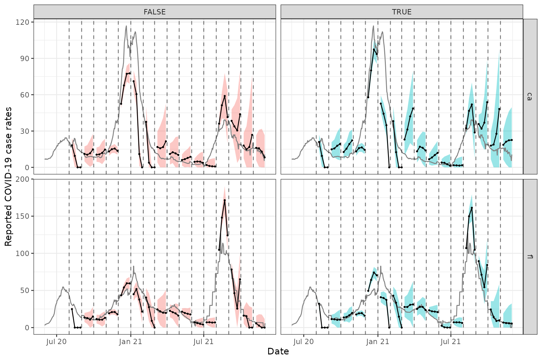
We can see that these forecasts, which come from training an ARX model jointly over CA and FL, exhibit generally less variability and wider prediction bands compared to the ones from the archive vignette, which come from training a separate ARX model on each state. As in the archive vignette, we can see a difference between version-aware (right column) and -unaware (left column) forecasting, as well.
Attribution
The case_rate_7d_av data used in this document is a
modified part of the COVID-19 Data
Repository by the Center for Systems Science and Engineering (CSSE) at
Johns Hopkins University as republished
in the COVIDcast Epidata API. This data set is licensed under the
terms of the Creative Commons
Attribution 4.0 International license by the Johns Hopkins
University on behalf of its Center for Systems Science in Engineering.
Copyright Johns Hopkins University 2020.
The percent_cli data is a modified part of the COVIDcast
Epidata API Doctor Visits data. This dataset is licensed under the
terms of the Creative Commons
Attribution 4.0 International license. Copyright Delphi Research
Group at Carnegie Mellon University 2020.