Work with archive objects and data revisions

In addition to the epi_df data structure, the epiprocess package has a companion structure called epi_archive. In comparison to an epi_df object, which can be seen as storing a single snapshot of a data set with the most up-to-date signal values as of some given time, an epi_archive object stores the full version history of a data set. Many signals of interest for epidemiological tracking are subject to revision (some more than others) and paying attention to data revisions can be important for all sorts of downstream data analysis and modeling tasks.

This vignette walks through working with epi_archive() objects and demonstrates some of their key functionality. We’ll work with a signal on the percentage of doctor’s visits with CLI (COVID-like illness) computed from medical insurance claims, available through the COVIDcast API. This signal is subject to very heavy and regular revision; you can read more about it on its API documentation page.

library(epidatr)
library(epiprocess)
library(data.table)
library(dplyr)
library(purrr)
library(ggplot2)

dv <- pub_covidcast(
  source = "doctor-visits",
  signals = "smoothed_adj_cli",
  geo_type = "state",
  time_type = "day",
  geo_values = "ca,fl,ny,tx",
  time_values = epirange(20200601, 20211201),
  issues = epirange(20200601, 20211201)
)

Getting data into `epi_archive` format

An epi_archive() object can be constructed from a data frame, data table, or tibble, provided that it has (at least) the following columns:

geo_value: the geographic value associated with each row of measurements.
time_value: the time value associated with each row of measurements.
version: the time value specifying the version for each row of measurements. For example, if in a given row the version is January 15, 2022 and time_value is January 14, 2022, then this row contains the measurements of the data for January 14, 2022 that were available one day later.

As we can see from the above, the data frame returned by epidatr::pub_covidcast() has the columns required for the epi_archive format, with issue playing the role of version. We can now use as_epi_archive() to bring it into epi_archive format. For removal of redundant version updates in as_epi_archive using compactify, please refer to the compactify vignette.

x <- dv %>%
  select(geo_value, time_value, version = issue, percent_cli = value) %>%
  as_epi_archive(compactify = TRUE)

class(x)

## [1] "epi_archive"

print(x)

## → An `epi_archive` object, with metadata:
## ℹ Min/max time values: 2020-06-01 / 2021-11-30
## ℹ First/last version with update: 2020-06-02 / 2021-12-01
## ℹ Versions end: 2021-12-01
## ℹ A preview of the table (119316 rows x 4 columns):
## Key: <geo_value, time_value, version>
##         geo_value time_value    version percent_cli
##            <char>     <Date>     <Date>       <num>
##      1:        ca 2020-06-01 2020-06-02          NA
##      2:        ca 2020-06-01 2020-06-06    2.140116
##      3:        ca 2020-06-01 2020-06-08    2.140379
##      4:        ca 2020-06-01 2020-06-09    2.114430
##      5:        ca 2020-06-01 2020-06-10    2.133677
##     ---                                            
## 119312:        tx 2021-11-26 2021-11-29    1.858596
## 119313:        tx 2021-11-27 2021-11-28          NA
## 119314:        tx 2021-11-28 2021-11-29          NA
## 119315:        tx 2021-11-29 2021-11-30          NA
## 119316:        tx 2021-11-30 2021-12-01          NA

An epi_archive is consists of a primary field DT, which is a data table (from the data.table package) that has the columns geo_value, time_value, version (and possibly additional ones), and other metadata fields, such as geo_type.

class(x$DT)

## [1] "data.table" "data.frame"

head(x$DT)

## Key: <geo_value, time_value, version>
##    geo_value time_value    version percent_cli
##       <char>     <Date>     <Date>       <num>
## 1:        ca 2020-06-01 2020-06-02          NA
## 2:        ca 2020-06-01 2020-06-06    2.140116
## 3:        ca 2020-06-01 2020-06-08    2.140379
## 4:        ca 2020-06-01 2020-06-09    2.114430
## 5:        ca 2020-06-01 2020-06-10    2.133677
## 6:        ca 2020-06-01 2020-06-11    2.197207

The variables geo_value, time_value, version serve as key variables for the data table, as well as any other specified in the metadata (described below). There can only be a single row per unique combination of key variables, and therefore the key variables are critical for figuring out how to generate a snapshot of data from the archive, as of a given version (also described below).

key(x$DT)

## [1] "geo_value"  "time_value" "version"

In general, the last version of each observation is carried forward (LOCF) to fill in data between recorded versions.

Some details on metadata

The following pieces of metadata are included as fields in an epi_archive object:

geo_type: the type for the geo values.

Metadata for an epi_archive object x can be accessed (and altered) directly, as in x$geo_type, etc. Just like as_epi_df(), the function as_epi_archive() attempts to guess metadata fields when an epi_archive object is instantiated, if they are not explicitly specified in the function call (as it did in the case above).

Summarizing Revision Behavior

There are many ways to examine the ways that signals change across different revisions. The simplest that is included directly in epiprocess is revision_summary(), which computes simple summary statistics for each key (by default, (geo_value,time_value) pairs), such as the lag to the first value (latency). In addition to the per key summary, it also returns an overall summary:

revision_details <- revision_summary(x, print_inform = TRUE)

## Min lag (time to first version):

##      min median     mean     max
##   3 days 3 days 3.5 days 12 days

## Fraction of epi_key+time_values with
## No revisions:
## • 0 out of 1,956 (0%)
## 
## Quick revisions (last revision within 3 days of the `time_value`):
## • 0 out of 1,956 (0%)
## 
## Few revisions (At most 3 revisions for that `time_value`):
## • 0 out of 1,956 (0%)
## 
## 
## Fraction of revised epi_key+time_values which have:
## Less than 0.1 spread in relative value:
## • 91 out of 1,956 (4.65%)
## 
## Spread of more than 2.22056495 in actual value (when revised):
## • 671 out of 1,956 (34.3%)
## 
## days until within 20% of the latest value:

##      min median     mean     max
##   3 days 5 days 9.1 days 67 days

So as was mentioned at the top, this is clearly a data set where basically everything has some amount of revisions, only 0.37% have no revision at all, and 0.92 have fewer than 3. Over 94% change by more than 10%. On the other hand, most are within plus or minus 20% within 5-9 days, so the revisions converge relatively quickly, even if the revisions continue for longer.

To do more detailed analysis than is possible with the above printing, we have revision_details:

revision_details %>%
  group_by(geo_value) %>%
  summarise(
    n_rev = mean(n_revisions),
    min_lag = min(min_lag),
    max_lag = max(max_lag),
    spread = mean(spread),
    rel_spread = mean(rel_spread),
    time_near_latest = mean(time_near_latest)
  )

## # A tibble: 4 × 7
##   geo_value n_rev min_lag max_lag spread rel_spread time_near_latest
##   <chr>     <dbl> <drtn>  <drtn>   <dbl>      <dbl> <drtn>          
## 1 ca         56.4 3 days  74 days   2.53      0.304 11.278119 days  
## 2 fl         56.4 3 days  74 days   2.29      0.280 10.830266 days  
## 3 ny         56.4 3 days  74 days   1.98      0.206  6.977505 days  
## 4 tx         56.4 3 days  74 days   1.63      0.218  7.398773 days

Most of the states have similar stats on most of these features, except for Florida, which takes nearly double the amount of time to get close to the right value, with California not too far behind.

Producing snapshots in `epi_df` form

A key method of an epi_archive class is epix_as_of(), which generates a snapshot of the archive in epi_df format. This represents the most up-to-date values of the signal variables as of a given version.

x_snapshot <- epix_as_of(x, as.Date("2021-06-01"))
class(x_snapshot)

## [1] "epi_df"     "tbl_df"     "tbl"        "data.frame"

head(x_snapshot)

## An `epi_df` object, 6 x 3 with metadata:
## * geo_type  = state
## * time_type = day
## * as_of     = 2021-06-01
## 
## # A tibble: 6 × 3
##   geo_value time_value percent_cli
## * <chr>     <date>           <dbl>
## 1 ca        2020-06-01        2.75
## 2 ca        2020-06-02        2.57
## 3 ca        2020-06-03        2.48
## 4 ca        2020-06-04        2.41
## 5 ca        2020-06-05        2.57
## 6 ca        2020-06-06        2.63

max(x_snapshot$time_value)

## [1] "2021-05-31"

attributes(x_snapshot)$metadata$as_of

## [1] "2021-06-01"

We can see that the max time value in the epi_df object x_snapshot that was generated from the archive is May 29, 2021, even though the specified version date was June 1, 2021. From this we can infer that the doctor’s visits signal was 2 days latent on June 1. Also, we can see that the metadata in the epi_df object has the version date recorded in the as_of field.

Below, we pull several snapshots from the archive, spaced one month apart. We overlay the corresponding signal curves as colored lines, with the version dates marked by dotted vertical lines, and draw the latest curve in black (from the latest snapshot x_latest that the archive can provide).

theme_set(theme_bw())

x_latest <- epix_as_of(x, x$versions_end)
self_max <- max(x$DT$version)
versions <- seq(as.Date("2020-06-01"), self_max - 1, by = "1 month")
snapshots <- map_dfr(versions, function(v) {
  epix_as_of(x, v) %>% mutate(version = v)
}) %>%
  bind_rows(
    x_latest %>% mutate(version = self_max)
  ) %>%
  mutate(latest = version == self_max)

ggplot(
  snapshots %>% filter(!latest),
  aes(x = time_value, y = percent_cli)
) +
  geom_line(aes(color = factor(version)), na.rm = TRUE) +
  geom_vline(aes(color = factor(version), xintercept = version), lty = 2) +
  facet_wrap(~geo_value, scales = "free_y", ncol = 1) +
  scale_x_date(minor_breaks = "month", date_labels = "%b %y") +
  labs(x = "Date", y = "% of doctor's visits with CLI") +
  theme(legend.position = "none") +
  geom_line(
    data = snapshots %>% filter(latest),
    aes(x = time_value, y = percent_cli),
    inherit.aes = FALSE, color = "black", na.rm = TRUE
  )

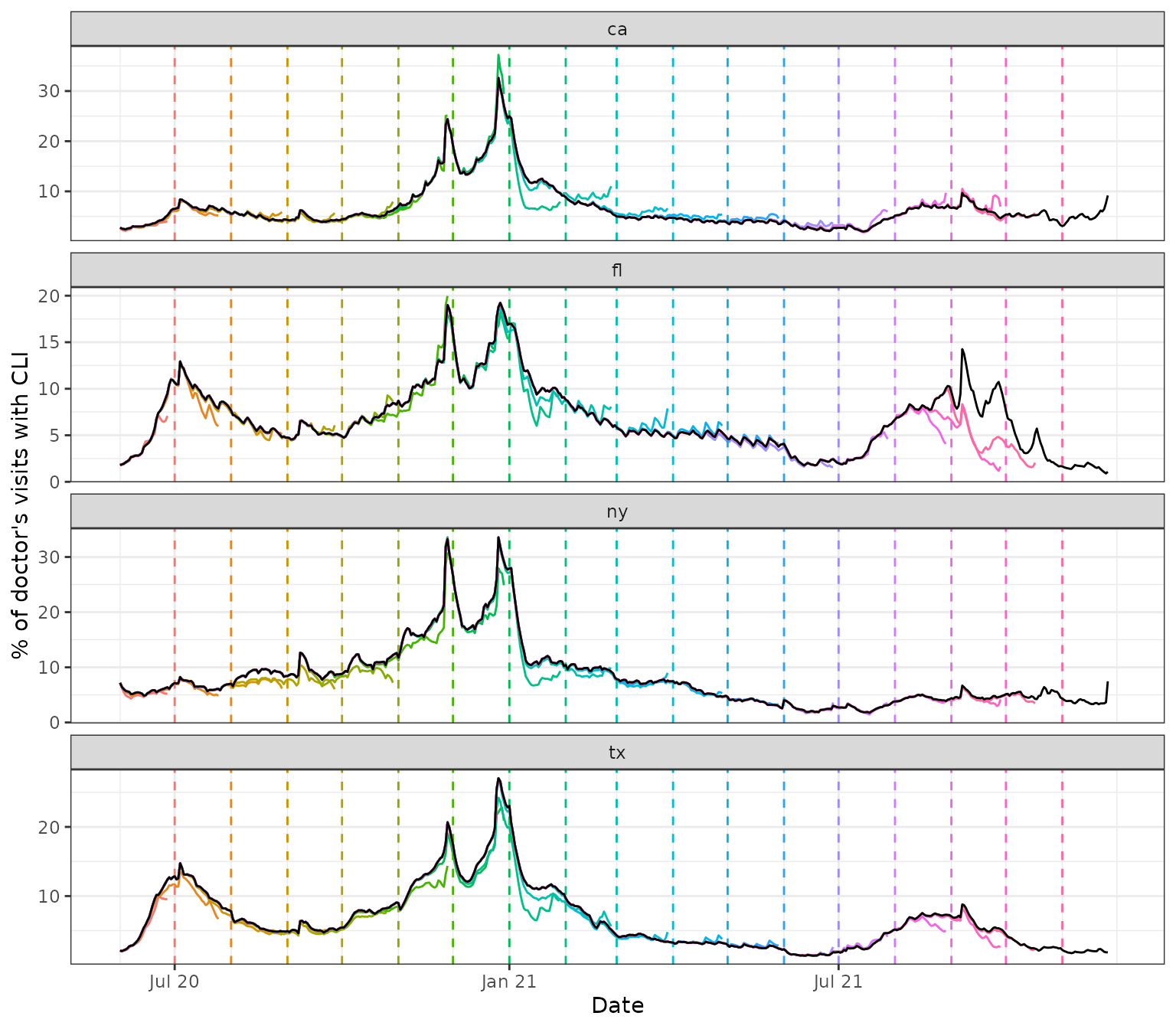
We can see some interesting and highly nontrivial revision behavior: at some points in time the provisional data snapshots grossly underestimate the latest curve (look in particular at Florida close to the end of 2021), and at others they overestimate it (both states towards the beginning of 2021), though not quite as dramatically. Modeling the revision process, which is often called backfill modeling, is an important statistical problem in it of itself.

Merging `epi_archive` objects

Now we demonstrate how to merge two epi_archive objects together, e.g., so that grabbing data from multiple sources as of a particular version can be performed with a single epix_as_of call. The function epix_merge() is made for this purpose. Below we merge the working epi_archive of versioned percentage CLI from outpatient visits to another one of versioned COVID-19 case reporting data, which we fetch the from the COVIDcast API, on the rate scale (counts per 100,000 people in the population).

When merging archives, unless the archives have identical data release patterns, NAs can be introduced in the non-key variables for a few reasons: - to represent the “value” of an observation before its initial release (when we need to pair it with additional observations from the other archive that have been released) - to represent the “value” of an observation that has no recorded versions at all (in the same sort of situation) - if requested via sync="na", to represent potential update data that we do not yet have access to (e.g., due to encountering issues while attempting to download the currently available version data for one of the archives, but not the other).

y <- pub_covidcast(
  source = "jhu-csse",
  signals = "confirmed_7dav_incidence_prop",
  geo_type = "state",
  time_type = "day",
  geo_values = "ca,fl,ny,tx",
  time_values = epirange(20200601, 20211201),
  issues = epirange(20200601, 20211201)
) %>%
  select(geo_value, time_value, version = issue, case_rate_7d_av = value) %>%
  as_epi_archive(compactify = TRUE)

x <- epix_merge(x, y, sync = "locf", compactify = TRUE)
print(x)
head(x$DT)

## → An `epi_archive` object, with metadata:
## ℹ Min/max time values: 2020-06-01 / 2021-11-30
## ℹ First/last version with update: 2020-06-02 / 2021-12-01
## ℹ Versions end: 2021-12-01
## ℹ A preview of the table (129638 rows x 5 columns):
## Key: <geo_value, time_value, version>
##         geo_value time_value    version percent_cli case_rate_7d_av
##            <char>     <Date>     <Date>       <num>           <num>
##      1:        ca 2020-06-01 2020-06-02          NA        6.628329
##      2:        ca 2020-06-01 2020-06-06    2.140116        6.628329
##      3:        ca 2020-06-01 2020-06-07    2.140116        6.628329
##      4:        ca 2020-06-01 2020-06-08    2.140379        6.628329
##      5:        ca 2020-06-01 2020-06-09    2.114430        6.628329
##     ---                                                            
## 129634:        tx 2021-11-26 2021-11-29    1.858596        7.957657
## 129635:        tx 2021-11-27 2021-11-28          NA        7.174299
## 129636:        tx 2021-11-28 2021-11-29          NA        6.834681
## 129637:        tx 2021-11-29 2021-11-30          NA        8.841247
## 129638:        tx 2021-11-30 2021-12-01          NA        9.566218

## Key: <geo_value, time_value, version>
##    geo_value time_value    version percent_cli case_rate_7d_av
##       <char>     <Date>     <Date>       <num>           <num>
## 1:        ca 2020-06-01 2020-06-02          NA        6.628329
## 2:        ca 2020-06-01 2020-06-06    2.140116        6.628329
## 3:        ca 2020-06-01 2020-06-07    2.140116        6.628329
## 4:        ca 2020-06-01 2020-06-08    2.140379        6.628329
## 5:        ca 2020-06-01 2020-06-09    2.114430        6.628329
## 6:        ca 2020-06-01 2020-06-10    2.133677        6.628329

Sliding version-aware computations

Lastly, we demonstrate another key method for archives, which is the epix_slide(). It works just like epi_slide() does for an epi_df object, but with one key difference: it performs version-aware computations. That is, for the computation at any given reference time t, it only uses data that would have been available as of t.

For the demonstration, we’ll revisit the forecasting example from the slide vignette, and now we’ll build a forecaster that uses properly-versioned data (that would have been available in real-time) to forecast future COVID-19 case rates from current and past COVID-19 case rates, as well as current and past values of the outpatient CLI signal from medical claims. We’ll extend the prob_ar() function from the slide vignette to accomodate exogenous variables in the autoregressive model, which is often referred to as an ARX model.

prob_arx <- function(x, y, lags = c(0, 7, 14), ahead = 7, min_train_window = 20,
                     lower_level = 0.05, upper_level = 0.95, symmetrize = TRUE,
                     intercept = FALSE, nonneg = TRUE) {
  # Return NA if insufficient training data
  if (length(y) < min_train_window + max(lags) + ahead) {
    return(data.frame(point = NA, lower = NA, upper = NA))
  }

  # Useful transformations
  if (!missing(x)) {
    x <- data.frame(x, y)
  } else {
    x <- data.frame(y)
  }
  if (!is.list(lags)) lags <- list(lags)
  lags <- rep(lags, length.out = ncol(x))

  # Build features and response for the AR model, and then fit it
  dat <- do.call(
    data.frame,
    unlist( # Below we loop through and build the lagged features
      purrr::map(seq_len(ncol(x)), function(i) {
        purrr::map(lags[[i]], function(j) lag(x[, i], n = j))
      }),
      recursive = FALSE
    )
  )
  names(dat) <- paste0("x", seq_len(ncol(dat)))
  if (intercept) dat$x0 <- rep(1, nrow(dat))
  dat$y <- lead(y, n = ahead)
  obj <- lm(y ~ . + 0, data = dat)

  # Use LOCF to fill NAs in the latest feature values, make a prediction
  setDT(dat)
  setnafill(dat, type = "locf")
  point <- predict(obj, newdata = tail(dat, 1))

  # Compute a band
  r <- residuals(obj)
  s <- ifelse(symmetrize, -1, NA) # Should the residuals be symmetrized?
  q <- quantile(c(r, s * r), probs = c(lower_level, upper_level), na.rm = TRUE)
  lower <- point + q[1]
  upper <- point + q[2]

  # Clip at zero if we need to, then return
  if (nonneg) {
    point <- max(point, 0)
    lower <- max(lower, 0)
    upper <- max(upper, 0)
  }
  return(data.frame(point = point, lower = lower, upper = upper))
}

Next we slide this forecaster over the working epi_archive object, in order to forecast COVID-19 case rates 7 days into the future.

fc_time_values <- seq(as.Date("2020-08-01"), as.Date("2021-11-30"), by = "1 month")

z <- x %>%
  group_by(geo_value) %>%
  epix_slide(
    fc = prob_arx(x = percent_cli, y = case_rate_7d_av, ahead = 7),
    .before = 119,
    .versions = fc_time_values
  ) %>%
  ungroup()

head(z, 10)

## # A tibble: 10 × 3
##    geo_value version    fc$point $lower $upper
##    <chr>     <date>        <dbl>  <dbl>  <dbl>
##  1 ca        2020-08-01    21.0   19.1   23.0 
##  2 fl        2020-08-01    44.5   38.9   50.0 
##  3 ny        2020-08-01     3.10   2.89   3.31
##  4 tx        2020-08-01    35.5   33.6   37.4 
##  5 ca        2020-09-01    22.9   20.1   25.8 
##  6 fl        2020-09-01    15.5   10.5   20.6 
##  7 ny        2020-09-01     3.16   2.93   3.39
##  8 tx        2020-09-01    17.5   14.3   20.7 
##  9 ca        2020-10-01    12.8    9.21  16.5 
## 10 fl        2020-10-01    14.7    8.72  20.6

We get back a tibble z with the grouping variables (here geo value), the (reference) time values, and a [“packed”][tidyr::pack] data frame column fc containing fc$point, fc$lower, and fc$upper that correspond to the point forecast, and the lower and upper endpoints of the 95% prediction band, respectively. (We could also have used , prob_ar(cases_7dav) to get three separate columns point, lower, and upper, or used fc = list(prob_ar(cases_7dav)) to make an fc column with a [“nested”][tidyr::nest] format (list of data frames) instead.)

On the whole, epix_slide() works similarly to epix_slide(), though there are a few notable differences, even apart from the version-aware aspect. You can read the documentation for epix_slide() for details.

We finish off by comparing version-aware and -unaware forecasts at various points in time and forecast horizons. The former comes from using epix_slide() with the epi_archive object x, and the latter from applying epi_slide() to the latest snapshot of the data x_latest.

x_latest <- epix_as_of(x, x$versions_end)

# Simple function to produce forecasts k weeks ahead
forecast_k_week_ahead <- function(x, ahead = 7, as_of = TRUE) {
  if (as_of) {
    x %>%
      group_by(geo_value) %>%
      epix_slide(
        fc = prob_arx(.data$percent_cli, .data$case_rate_7d_av, ahead = ahead), .before = 119,
        .versions = fc_time_values
      ) %>%
      mutate(target_date = .data$version + ahead, as_of = TRUE) %>%
      ungroup()
  } else {
    x_latest %>%
      group_by(geo_value) %>%
      epi_slide(
        fc = prob_arx(.data$percent_cli, .data$case_rate_7d_av, ahead = ahead), .window_size = 120,
        .ref_time_values = fc_time_values
      ) %>%
      mutate(target_date = .data$time_value + ahead, as_of = FALSE) %>%
      ungroup()
  }
}

# Generate the forecasts, and bind them together
fc <- bind_rows(
  forecast_k_week_ahead(x, ahead = 7, as_of = TRUE),
  forecast_k_week_ahead(x, ahead = 14, as_of = TRUE),
  forecast_k_week_ahead(x, ahead = 21, as_of = TRUE),
  forecast_k_week_ahead(x, ahead = 28, as_of = TRUE),
  forecast_k_week_ahead(x, ahead = 7, as_of = FALSE),
  forecast_k_week_ahead(x, ahead = 14, as_of = FALSE),
  forecast_k_week_ahead(x, ahead = 21, as_of = FALSE),
  forecast_k_week_ahead(x, ahead = 28, as_of = FALSE)
)

# Plot them, on top of latest COVID-19 case rates
ggplot(fc, aes(x = target_date, group = time_value, fill = as_of)) +
  geom_ribbon(aes(ymin = fc$lower, ymax = fc$upper), alpha = 0.4) +
  geom_line(
    data = x_latest, aes(x = time_value, y = case_rate_7d_av),
    inherit.aes = FALSE, color = "gray50"
  ) +
  geom_line(aes(y = fc$point)) +
  geom_point(aes(y = fc$point), size = 0.5) +
  geom_vline(aes(xintercept = time_value), linetype = 2, alpha = 0.5) +
  facet_grid(vars(geo_value), vars(as_of), scales = "free") +
  scale_x_date(minor_breaks = "month", date_labels = "%b %y") +
  labs(x = "Date", y = "Reported COVID-19 case rates") +
  theme(legend.position = "none")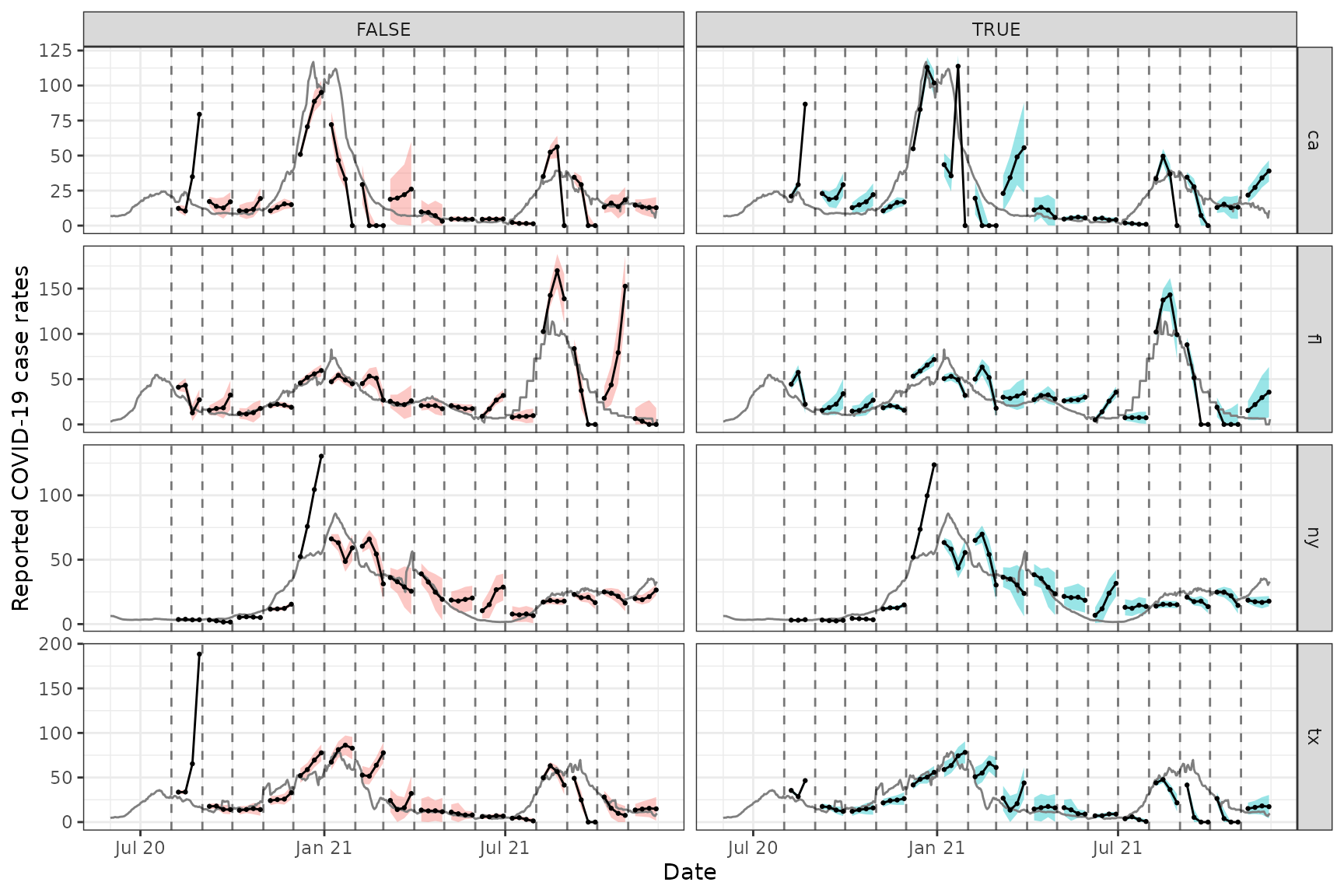

Each row displays the forecasts for a different location (CA, FL, NY, and TX), and each column corresponds to whether properly-versioned data is used (FALSE means no, and TRUE means yes). We can see that the properly-versioned forecaster is, at some points in time, more problematic; for example, it massively overpredicts the peak in both locations in winter wave of 2020. However, performance is pretty poor across the board here, whether or not properly-versioned data is used. Similar to what we saw in the slide vignette, the ARX forecasts can too volatile, overconfident, or both.

Some of the volatility can be attenuated here by training an ARX model jointly over locations; the advanced sliding vignette gives a demonstration of how to do this. But really, the epipredict package, which builds off the data structures and functionality in the current package, is the place to look for more robust forecasting methodology. The forecasters that appear in the vignettes in the current package are only meant to demo the slide functionality with some of the most basic forecasting methodology possible.

Sliding version-aware computations with geo-pooling

First, we fetch the versioned data and build the archive.

library(epidatr)
library(data.table)
library(ggplot2)
theme_set(theme_bw())

y1 <- pub_covidcast(
  source = "doctor-visits",
  signals = "smoothed_adj_cli",
  geo_type = "state",
  time_type = "day",
  geo_values = "ca,fl",
  time_values = epirange(20200601, 20211201),
  issues = epirange(20200601, 20211201)
)

y2 <- pub_covidcast(
  source = "jhu-csse",
  signal = "confirmed_7dav_incidence_prop",
  geo_type = "state",
  time_type = "day",
  geo_values = "ca,fl",
  time_values = epirange(20200601, 20211201),
  issues = epirange(20200601, 20211201)
)

x <- y1 %>%
  select(geo_value, time_value,
    version = issue,
    percent_cli = value
  ) %>%
  as_epi_archive(compactify = FALSE)

# mutating merge operation:
x <- epix_merge(
  x,
  y2 %>%
    select(geo_value, time_value,
      version = issue,
      case_rate_7d_av = value
    ) %>%
    as_epi_archive(compactify = FALSE),
  sync = "locf",
  compactify = FALSE
)

Next, we extend the ARX function to handle multiple geo values, since in the present case, we will not be grouping by geo value and each slide computation will be run on multiple geo values at once. Note that, because epix_slide() only returns the grouping variables, time_value, and the slide computations in the eventual returned tibble, we need to include geo_value as a column in the output data frame from our ARX computation.

library(tidyr)
library(purrr)

prob_arx_args <- function(lags = c(0, 7, 14),
                          ahead = 7,
                          min_train_window = 20,
                          lower_level = 0.05,
                          upper_level = 0.95,
                          symmetrize = TRUE,
                          intercept = FALSE,
                          nonneg = TRUE) {
  return(list(
    lags = lags,
    ahead = ahead,
    min_train_window = min_train_window,
    lower_level = lower_level,
    upper_level = upper_level,
    symmetrize = symmetrize,
    intercept = intercept,
    nonneg = nonneg
  ))
}

prob_arx <- function(x, y, geo_value, time_value, args = prob_arx_args()) {
  # Return NA if insufficient training data
  if (length(y) < args$min_train_window + max(args$lags) + args$ahead) {
    return(data.frame(
      geo_value = unique(geo_value), # Return geo value!
      point = NA, lower = NA, upper = NA
    ))
  }

  # Set up x, y, lags list
  if (!missing(x)) {
    x <- data.frame(x, y)
  } else {
    x <- data.frame(y)
  }
  if (!is.list(args$lags)) args$lags <- list(args$lags)
  args$lags <- rep(args$lags, length.out = ncol(x))

  # Build features and response for the AR model, and then fit it
  dat <- tibble(i = seq_len(ncol(x)), lag = args$lags) %>%
    unnest(lag) %>%
    mutate(name = paste0("x", seq_len(nrow(.)))) %>% # nolint: object_usage_linter
    # One list element for each lagged feature
    pmap(function(i, lag, name) {
      tibble(
        geo_value = geo_value,
        time_value = time_value + lag, # Shift back
        !!name := x[, i]
      )
    }) %>%
    # One list element for the response vector
    c(list(
      tibble(
        geo_value = geo_value,
        time_value = time_value - args$ahead, # Shift forward
        y = y
      )
    )) %>%
    # Combine them together into one data frame
    reduce(full_join, by = c("geo_value", "time_value")) %>%
    arrange(time_value)
  if (args$intercept) dat$x0 <- rep(1, nrow(dat))
  obj <- lm(y ~ . + 0, data = select(dat, -geo_value, -time_value))

  # Use LOCF to fill NAs in the latest feature values (do this by geo value)
  setDT(dat) # Convert to a data.table object by reference
  cols <- setdiff(names(dat), c("geo_value", "time_value"))
  dat[, (cols) := nafill(.SD, type = "locf"), .SDcols = cols, by = "geo_value"]

  # Make predictions
  test_time_value <- max(time_value)
  point <- predict(
    obj,
    newdata = dat %>%
      dplyr::group_by(geo_value) %>%
      dplyr::filter(time_value == test_time_value)
  )

  # Compute bands
  r <- residuals(obj)
  s <- ifelse(args$symmetrize, -1, NA) # Should the residuals be symmetrized?
  q <- quantile(c(r, s * r), probs = c(args$lower, args$upper), na.rm = TRUE)
  lower <- point + q[1]
  upper <- point + q[2]

  # Clip at zero if we need to, then return
  if (args$nonneg) {
    point <- pmax(point, 0)
    lower <- pmax(lower, 0)
    upper <- pmax(upper, 0)
  }
  return(data.frame(
    geo_value = unique(geo_value), # Return geo value!
    point = point, lower = lower, upper = upper
  ))
}

We now make forecasts on the archive and compare to forecasts on the latest data.

# Latest snapshot of data, and forecast dates
x_latest <- epix_as_of(x, version = max(x$DT$version))
fc_time_values <- seq(as.Date("2020-08-01"),
  as.Date("2021-11-30"),
  by = "1 month"
)

# Simple function to produce forecasts k weeks ahead
forecast_k_week_ahead <- function(x, ahead = 7, as_of = TRUE) {
  if (as_of) {
    x %>%
      epix_slide(
        fc = prob_arx(.data$percent_cli, .data$case_rate_7d_av, .data$geo_value, .data$time_value,
          args = prob_arx_args(ahead = ahead)
        ),
        .before = 219, .versions = fc_time_values
      ) %>%
      mutate(
        target_date = .data$version + ahead, as_of = TRUE,
        geo_value = .data$fc$geo_value
      )
  } else {
    x_latest %>%
      epi_slide(
        fc = prob_arx(.data$percent_cli, .data$case_rate_7d_av, .data$geo_value, .data$time_value,
          args = prob_arx_args(ahead = ahead)
        ),
        .window_size = 220, .ref_time_values = fc_time_values
      ) %>%
      mutate(target_date = .data$time_value + ahead, as_of = FALSE)
  }
}

# Generate the forecasts, and bind them together
fc <- bind_rows(
  forecast_k_week_ahead(x, ahead = 7, as_of = TRUE),
  forecast_k_week_ahead(x, ahead = 14, as_of = TRUE),
  forecast_k_week_ahead(x, ahead = 21, as_of = TRUE),
  forecast_k_week_ahead(x, ahead = 28, as_of = TRUE),
  forecast_k_week_ahead(x, ahead = 7, as_of = FALSE),
  forecast_k_week_ahead(x, ahead = 14, as_of = FALSE),
  forecast_k_week_ahead(x, ahead = 21, as_of = FALSE),
  forecast_k_week_ahead(x, ahead = 28, as_of = FALSE)
)

# Plot them, on top of latest COVID-19 case rates
ggplot(fc, aes(x = target_date, group = time_value, fill = as_of)) +
  geom_ribbon(aes(ymin = fc$lower, ymax = fc$upper), alpha = 0.4) +
  geom_line(
    data = x_latest, aes(x = time_value, y = case_rate_7d_av),
    inherit.aes = FALSE, color = "gray50"
  ) +
  geom_line(aes(y = fc$point)) +
  geom_point(aes(y = fc$point), size = 0.5) +
  geom_vline(aes(xintercept = time_value), linetype = 2, alpha = 0.5) +
  facet_grid(vars(geo_value), vars(as_of), scales = "free") +
  scale_x_date(minor_breaks = "month", date_labels = "%b %y") +
  labs(x = "Date", y = "Reported COVID-19 case rates") +
  theme(legend.position = "none")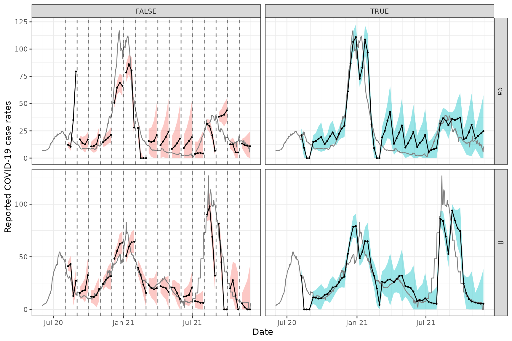

We can see that these forecasts, which come from training an ARX model jointly over CA and FL, exhibit generally less variability and wider prediction bands compared to the ones from the archive vignette, which come from training a separate ARX model on each state. As in the archive vignette, we can see a difference between version-aware (right column) and -unaware (left column) forecasting, as well.

Attribution

This document contains a dataset that is a modified part of the COVID-19 Data Repository by the Center for Systems Science and Engineering (CSSE) at Johns Hopkins University as republished in the COVIDcast Epidata API. This data set is licensed under the terms of the Creative Commons Attribution 4.0 International license by the Johns Hopkins University on behalf of its Center for Systems Science in Engineering. Copyright Johns Hopkins University 2020.

The percent_cli data is a modified part of the COVIDcast Epidata API Doctor Visits data. This dataset is licensed under the terms of the Creative Commons Attribution 4.0 International license. Copyright Delphi Research Group at Carnegie Mellon University 2020.

Getting data into epi_archive format